Cholesky decomposition a tool with many uses Tony

Cholesky decomposition – a tool with many uses Tony O’Hagan, Leo Bastos MUCM/SAMSI, April 07 Slide 1

Prununciation n Cholesky was French … n Sholesky n But his name is probably Polish … n Kholesky n Or maybe Russian … n Sholesky or n Kholesky or n Tsholesky n Take your pick!! http: //mucm. group. shef. ac. uk Slide 2

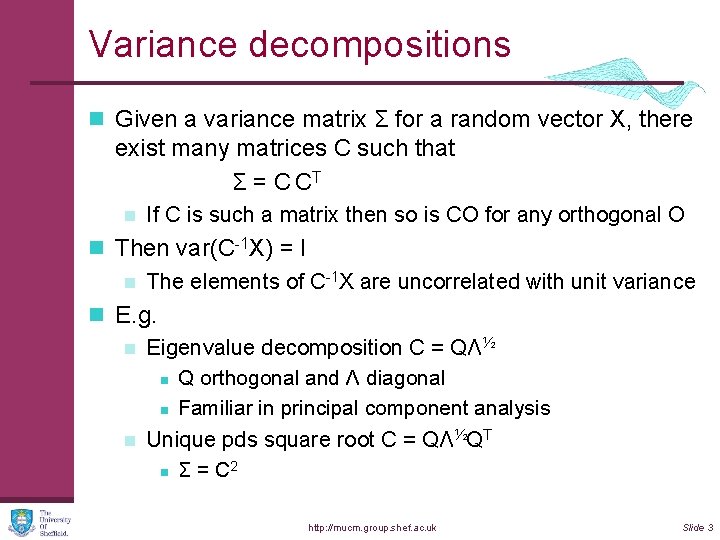
Variance decompositions n Given a variance matrix Σ for a random vector X, there exist many matrices C such that Σ = C CT n If C is such a matrix then so is CO for any orthogonal O n Then var(C-1 X) = I n The elements of C-1 X are uncorrelated with unit variance n E. g. n Eigenvalue decomposition C = QΛ½ n Q orthogonal and Λ diagonal n Familiar in principal component analysis n Unique pds square root C = QΛ½QT 2 n Σ = C http: //mucm. group. shef. ac. uk Slide 3

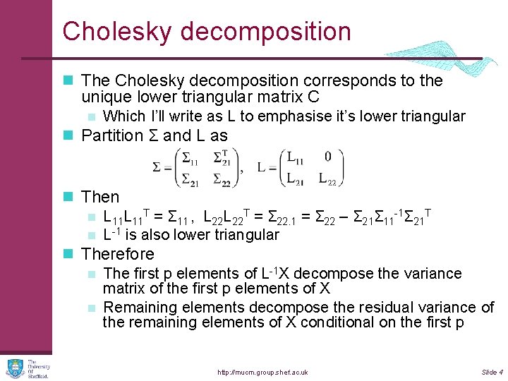
Cholesky decomposition n The Cholesky decomposition corresponds to the unique lower triangular matrix C n Which I’ll write as L to emphasise it’s lower triangular n Partition Σ and L as n Then n L 11 T = Σ 11 , L 22 T = Σ 22. 1 = Σ 22 – Σ 21Σ 11 -1Σ 21 T n L-1 is also lower triangular n Therefore n The first p elements of L-1 X decompose the variance matrix of the first p elements of X n Remaining elements decompose the residual variance of the remaining elements of X conditional on the first p http: //mucm. group. shef. ac. uk Slide 4

Computing Cholesky n Recursion; take p = 1 n L 11 = √(Σ 11) (scalar) n L 21 = Σ 21/L 21 (column vector divided by scalar) n L 22 is the Cholesky decomposition of Σ 22. 1 n Inverse matrix is usually computed in the same recursion n Much faster and more accurate than eigenvalue computation n Method of choice for inverting pds matrices http: //mucm. group. shef. ac. uk Slide 5

Principal Cholesky n There are many Cholesky decompositions n Permute the variables in X n Obviously gives different decomposition n Principal Cholesky decomposition (PCD) n At each step in recursion, permute to bring the largest diagonal element of Σ (or Σ 22. 1) to the first element n Analogous to principal components n First Cholesky component is the element of X with largest variance n Second is a linear combination of the first with the element with largest variance given the first n And so on http: //mucm. group. shef. ac. uk Slide 6

Numerical stability n Important when decomposing or inverting near- singular matrices n n A problem that arises routinely with Gaussian process methods I’ve been using PCD for this purpose for about 20 years n Division by √(Σ 11) is the major cause of instability n Rounding error magnified n Rounding error can even cause √(Σ 11) to be –ve n PCD postpones this problem to late stages of the recursion n n The whole of Σ 22. 1 is then small, and we can truncate Analogous to not using all the principal components http: //mucm. group. shef. ac. uk Slide 7

Fitting emulators n A key step in the fitting process is inverting the matrix A of covariances between the design points n Typically needs to be done many times n Problems arise when points are close together relative to correlation length parameters n n n A becomes ill-conditioned n E. g. points on trajectory of a dynamic model n Or in Herbie’s optimisation PCD allows us to identify redundant design points Simply discard them n But it’s important to check fit n Observed function values at discarded points should be consistent with the (narrow) prediction bounds given included points http: //mucm. group. shef. ac. uk Slide 8

Validating emulators n Having fitted the emulator, we test its predictions against new model runs n We can look at standardised residuals for individual predicted points n But these are correlated n Mahalanobis distance to test the whole set D = (y – m)TV-1(y – m) n n Where y is new data, m is mean vector and V is predictive variance matrix Approx χ2 with df equal to number of new points n Any decomposition of V decomposes D n Eigenvalues useful but may be hard to interpret http: //mucm. group. shef. ac. uk Slide 9

Validating emulators (2) n PCD keeps the focus on individual points, but conditions them on other points Initially picks up essentially independent points n Interest in later points, where variance is reduced conditional on other points n In principle, points with the smallest conditional variances may provide most stringent tests n n But may be badly affected by rounding error http: //mucm. group. shef. ac. uk Slide 10

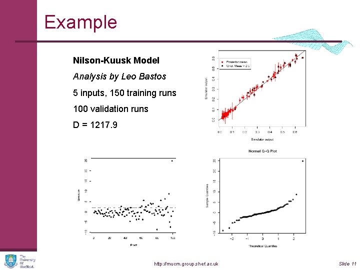
Example Nilson-Kuusk Model Analysis by Leo Bastos 5 inputs, 150 training runs 100 validation runs D = 1217. 9 http: //mucm. group. shef. ac. uk Slide 11

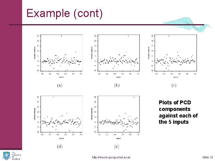
Example (cont) Plots of PCD components against each of the 5 inputs http: //mucm. group. shef. ac. uk Slide 12

Functional outputs n Various people have used principal components to do dimension reduction on functional or highly multivariate outputs n PCD selects instead a subset of points on the function (or individual outputs) Could save time if not all outputs are needed n Or save observations when calibrating n Helps with interpretation n Facilitates eliciting prior knowledge n http: //mucm. group. shef. ac. uk Slide 13

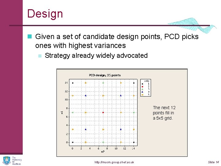
Design n Given a set of candidate design points, PCD picks ones with highest variances n Strategy already widely advocated Fourcome corners Next first. centres of the The next 12 sides. points fill in Then centre. a 5 x 5 Then thegrid. four blue points http: //mucm. group. shef. ac. uk Slide 14

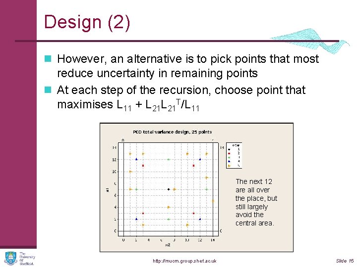
Design (2) n However, an alternative is to pick points that most reduce uncertainty in remaining points n At each step of the recursion, choose point that maximises L 11 + L 21 T/L 11 First in the 4 Next point we get the. The centre. next 12 green points are all over (notice first loss Then 4 points the place, but of symmetry). around it. still largely The four blue avoid the points are a central area. surprise! http: //mucm. group. shef. ac. uk Slide 15

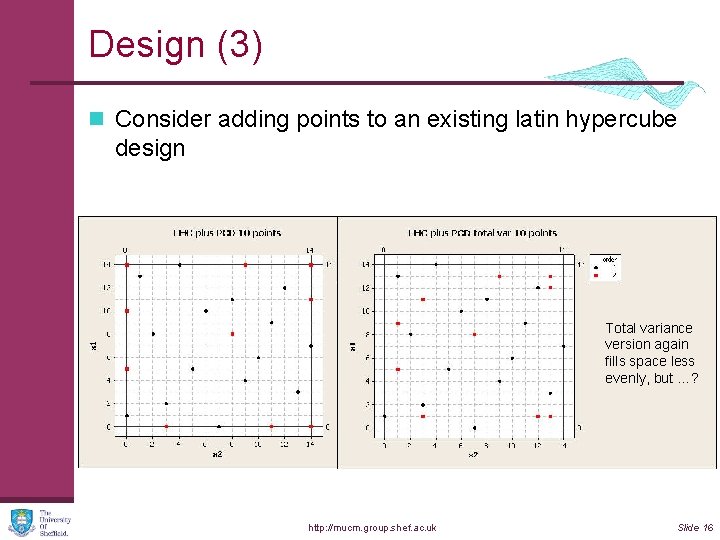
Design (3) n Consider adding points to an existing latin hypercube design Total variance version again fills space less evenly, but …? http: //mucm. group. shef. ac. uk Slide 16

Conclusion(s) I ♥ Cholesky! http: //mucm. group. shef. ac. uk Slide 17