Chapter Five Hydropower Systems Introduction Hydropower Engineering refers

Chapter Five Hydropower Systems

Introduction ØHydropower Engineering refers to the technology involved in converting the pressure energy and kinetic energy of water into more easily used electrical energy.

ØThe amount of water power developed from any stream, river or lake is a function of mainly: 1. The flow rate of water 2. The head that is available ØHydroelectric power and energy that can be generated in a hydropower plant is determined from: P = QHn E = QHn t ØWhere P is the power in k. W, is the specific weight of water in k. N/m 3, Q is the discharge in m 3/s, Hn is the net head (gross head minus hydraulic losses) in meters, is the overall efficiency (%), E is the hydroelectric energy in k. Wh and t is the time interval for power generation in hours.

Terminology and Turbine Types Terminology Ø Power capacity is often used in referring to the rated capability of the hydro plant to produce energy. Manufacturers of hydraulic turbines are usually required to specify what the rated capacity of their units is in either horsepower or kilowatts. Ø Demand Load • Demand refers' to the amount of power needed or desired; • load refers to the rate at which electrical energy is actually delivered to or by a system. In this context, load can include the output from several hydropower plants.

Ø Full gate Discharge : is the flow condition which prevails when turbine gates or valves are fully open. At maximum rated head and full gate, the maximum discharge will flow through the turbine. Ø Rated discharge refers to a gate opening or plant discharge which at rated head produces the rated power output of the turbine. Ø Hydraulic head is the elevation difference the water falls in passing through the plant. Ø Gross head of a hydropower facility is the difference between head water elevation and tail water elevation. (Headwater is the water in the forebay or impoundment supplying the turbine; tail water is the water issuing from the draft tube exit. )

Ø Net head is the effective head on the turbine and is equal to the gross head minus the hydraulic losses before entrance to the turbine and outlet losses. Ø Design head is the effective head for which the turbine is designed for best speed and efficiency. Ø Rated head is the lowest head at which the full-gate discharge of the turbine will produce the rated capacity of the generator. The term is sometimes used interchangeably with the term effective head. Ø Critical head is the net head or effective head at which fullgate output of the turbine produces the permissible overload on the generator at unit power factor. "Critical head" is used in studies of cavitation and turbine setting.

Components of Hydropower Plants Ø Most conventional hydroelectric components § Dam § Turbine § Generator § Transmission lines plants include four major Fig 1. 2 Major Components of a Conventional type of Hydropower Plant

Dam - Most hydropower plants rely on a dam that holds back water, creating a large reservoir. Often, this reservoir is used as a recreational Lake. Fig. 1. 3 Basic components of a conventional hydropower plant

Intake - Gates on the dam open and gravity pulls the water through the penstock, a pipeline that leads to the turbine. Water builds up pressure as it flows through this pipe. Turbine - The water strikes and turns the large blades of a turbine, which is attached to a generator above it by way of a shaft. Generators - As the turbine blades turn, so do a series of magnets inside the generator. Giant magnets rotate past copper coils, producing alternating current (AC) by moving electrons. Transformer - The transformer inside the powerhouse takes the AC and converts it to a higher- voltage current. Power lines - Out of every power plant come four wires: the three phases of power being produced simultaneously plus a neutral or ground common to all three.

Outflow - Used water is carried through pipelines, called tailraces, and re-enters the river downstream. Penstock pipe- The penstock pipe transports water under pressure from the forebay tank to the turbine, where the potential energy of the water is converted into kinetic energy in order to rotate the turbine. The hydropower plant components area is categorized as: • Civil works: Includes dam, powerhouse and spillway(structures used to provide for the controlled release of flows from a dam into a downstream area, typically being the river that was dammed) • Mechanical work: includes turbine, penstock, valves and gates • Electrical and other Equipments: includes transformer, generators and auxiliary equipments

Potential and Developed Hydropower Resources Ø Hydropower potential is generally evaluated in three categories, namely theoretical, technical and economical potential. Ø Theoretical potential is defined as the sum of the annual energy potentially available from all natural flows from the largest rivers to the smallest creek, regardless of the losses. Ø Technical potential is the part of theoretical potential which can be utilized with the current technology regardless of economic and other considerations. This definition of potential subtracts friction losses in water ways and efficiencies in the electromechanical equipment as well as the extreme low heads which are considered as infeasible.

ØEconomic potential is the part of the technical potential which can be regarded as economic when compared to alternative sources of power like oil and coal. ØIt is dependent on the cost of alternative sources. Therefore, it may change with time and should be updated regularly. ØUnion of the Electricity Industry uses a definition called exploitable hydropower potential for the portion of the economical potential which can be harnessed considering environmental and other special restrictions. • The Estimated total technical potential for hydropower in the world is as much as 15955 TWh/year or 4. 8 times greater than today's hydropower production.

The blue arrow represents a general historic increase in hydropower following growing demand for electricity worldwide. From 1999 through 2005 (illustrated by the orange arrow), hydropower development was largely halted worldwide, reflecting the impact of the World Commission on Dams (WCD), which was convened to review the development effectiveness of large dams and develop guidelines for the development of new dams. From 2005 onwards (green arrow), hydropower development has seen an upswing in development, which can be partly attributed to the impact of intensive efforts by the International Hydropower Association (IHA) and hydropower companies to negotiate sustainability guidelines for the sector. Figure 1. 6 – Global total hydropower generation since 1980

Classification of Hydro-Electric Power Plants Ø In studying the subject of hydropower engineering, it is important to understand the different types of development. Hydroelectric power plants can be classified in different ways according to their characteristics. Classification According to Operation Mode I. Impoundment Plants Ø Also called ‘storage plants’ or ‘reservoir plants’ is the most common type of hydroelectric power plants. These plants are usually large hydropower schemes and use a dam to store river water in a reservoir.

ØThese plants store water when the flows are relatively high and this storage compensates for the low-flow seasons. Therefore, a relatively constant supply of energy is maintained throughout a year. Fig 1. 7 Major parts of storage type of Hydropower Plant

II. Run-of-river Plants ØThis type of plant generally does not have a storage. By means of a diversion weir, water is diverted from the river and given to the transmission canal or sometimes tunnel. ØAt the end of the transmission canal lies a head pond or forebay facilitating a gentle approach to the intake of penstock. Forebays also serve in surge reduction and sediment removal. ØSince these plants do not have storage, energy generation is dependent on the flow in the river.

Ø General layout of run-of-river plants is given in figure below. Fig 1. 8 General layout of run- of-river plant

III. Pumped-Storage Plants ØIn contrast to conventional hydropower plants, pumped storage plants reuse water. They store electrical energy as potential energy. ØThey pump water to an upper reservoir at times of surplus energy on an electrical supply grid-typically, at night. This potential energy is then released through a hydro-electrical generator at times of high demand. Therefore, pumped-storage plants function like a large battery. ØThe combined use of pumped storage facilities with other types of electricity generation creates large cost savings through more efficient utilization of base-load plants.

ØGraphical representation of a pumped-storage plant is given in figure below. Fig 1. 9 General layout of pumped storage plant

Ø A basic function of pumped storage power stations is load leveling Fig 1. 10 Load Leveling in Pumped Storage Systems

Classification According to the Installed Capacity ØThere is no consensus in the world on the classification of hydropower plants according to installed capacity. They can be classified as large, small, mini, micro and pico hydropower plants. ØMini, micro and pico hydropower plants could be regarded as small hydro power plants; however, they have specific technical characteristics and deserve their own definition. • Different countries and organizations have different definitions. An example is the one made by Natural Resources Canada. According to this definition:

üMini hydropower 100 k. W to 1 MW üMicro hydropower 10 k. W to 100 k. W üPico hydropower less than 10 k. W Ethiopia also uses a classification of hydropower systems which differs from other countries, the Ethiopian definitions are follows: Terminology Capacity limits Unit Large >30 MW Medium 10 - 30 MW Small 1 - 10 MW Mini 501 - 1, 000 k. W Micro 11 - 500 k. W Pico ≤ 10 k. W Classification According to Operating Conditions I. Base Load Plants: These plants operate continuously at a nearly constant power and provide the power demand at base of the load curve (Fig. 1. 9). Storage type and run-of river plants can provide base load service. II. Peak Load Plants: These power plants are designed primarily for the purpose of supplying the peak load of a power system (Fig. 1. 9).

Pumped-storage plants are good examples of peak load plants. Storage type plants may also provide peak load service. Run-of-river plants can supply peak power only if they have a pond. Fig 1. 11 Typical daily load curve

Hydrologic Analysis of Hydropower Ø Hydrology is the study of the occurrence, movement, and distribution of water on, above, and within the earth's surface. Ø Parameters necessary in making hydropower studies are water discharge (Q) and hydraulic head (h). The measurement and analyses of these parameters are primarily hydrologic problems. Ø Determination of the head for a proposed hydropower plant is a surveying problem that identifies elevations of water surfaces as they are expected to exist during operation of the hydropower plant. Ø This implies that conceptualization has been made of where water will be directed from a water source and where the water will be discharged from a power plant.

Flow Duration Analysis Ø A useful way of treating the time variability of water discharge data in hydropower studies is by utilizing flow duration curves. Flow Duration Curves Ø is a plot of flow versus the percent of time a particular flow can be expected to be exceeded. Ø A flow duration curve merely reorders the flows in order of magnitude instead of the true time ordering of flows in a flow versus time plot. Ø A flow duration curve shows the relation between flows and lengths of time during which they are available.

Ø A typical flow duration curve is shown below Fig. 2. 3 Example of flow duration curve

Ø For environmental reasons, certain amount of flow is left in the river – Residual flow Qr. Ø Residual flow Qr must be subtracted from the flow duration curve for the calculation of plant capacity, firm capacity and the available energy. Ø Firm flow is flow available p% of the time, usually equal to 95%. It is calculated from the available flow duration curve. In Fig. 2. 3, firm flow is 1. 5 m 3/s with p set to 90% Ø Two methods are used for computing ordinates for flow duration curve – The rank ordered technique and – The class-interval technique

Ø The rank-ordered technique: considers a total time series of flows that represent equal increments of time for each measurement value, such as mean daily, weekly, or monthly flows, and ranks the flows according to magnitude. Ø The flow data are ranked according to magnitude (in descending order) and the frequency of occurrence, FX, is given by, FXm = (m/n) 100 FXm = (m/n + 1) 100 (California formula), or (Weibull formula) where, n = number of records, m = the order number in the rank (m = 1 for the highest ranked value), and FXm = frequency of occurrence (% dependable flow or the probability of flow being equaled or exceeded). ØThe flow value is then plotted versus the respective computed exceedance percentage. Ø Naturally, the longer the record, the more statistically valuable the information that results.

Example 2. Draw the flow duration curve for the following stream river flow using rank ordered technique. Month Flow (m 3/s) January 65 February 5 0 March 42 April 40 May 40 June 115 July 400 August 340 September 270 October 155 November 115 December 85 January 65

Solution M onth Flow (m 3/s) Rank Exceedence % January 65 8 66. . 67% February 50 9 75. 00% March 42 10 83. 33% April 40 12 100. 00% May 40 12 100. 00% June 115 6 50. 00% July 400 1 8. 33% August 340 2 16. 67% September 270 3 25. 00% October 155 4 33. 33% November 115 6 50. 00% December 85 7 58. 33%

FDC 450 400 Discharge m 3/s 350 300 250 200 150 100 50 0 0 20 40 60 Exceedence % 80 100 120

ØThe class-interval technique: is slightly different in that the time series of flow values are categorized into class intervals. ØThe classes range from the highest flow value to the lowest value in the time series. A tally is made of the number of flows in each, and by summation the number of values greater than a given upper limit of the class can be determined. ØThe number of flows greater than the upper limit of a class interval can be divided by the total number of flow values in the data series to obtain the exceedance percentage. ØThe value of the flow for the particular upper limit of the class interval is then plotted versus the computed exceedance percent.

Example 3 Monthly Flow Data Using the data in table above plot the flow duration curve using class interval method

Solution the relative and the cumulative relative frequencies for a class interval of 5 cumecs are as given in Table below.

Energy and power analysis using a flow duration approach • When a run-of river type of power study is done and a flow duration analysis is used, the capacity or size of hydropower units determines the maximum amount of water that will go through the unit or units. This is dictated by the nominal runner diameter and the accompanying outlet area and draft tube. • A flow duration curve is used to explain discharge capacity, Qc, as labeled in the Figure. This Qc, is the discharge at full gate opening of the runner under design head.

ØEven though to the left of that point on the duration curve the stream discharge is greater, it is not possible to pass the higher discharges through the plant. If the reservoir or pondage is full, water must be bypassed by a spillway. ØIf hydraulic head and the expected losses in the penstock are known, it is possible to generate a power duration curve from the flow duration curve. The Pc value of power is the fullgate discharge value of power. Energy production for a year or a time period is the product of the power ordinate and time and is thus the area under the power duration curve multiplied by an appropriate conversion factor.

ØIt should be noted that to the left of the power capacity point the power tends to decrease. This is due to the fact that net head available is decreasing due to a rising tail water caused by the higher flows that are occurring during that time interval or exceedance period. Ø While plotting the Power duration curve the actual output is diminished by the fact that the turbine has losses in transforming the potential and kinetic energy into mechanical energy. Thus an efficiency term must be introduced to give the standard power equation:

Exercise-1: draw the power duration curve for the following river stream flow. Take, Qc = 270 m 3/s Month Flow (m 3/s) Head(m) E fficiency January 65 83. 5 0. 87 February 50 83. 5 0. 83 March 42 83. 5 0. 75 April 40 83. 5 0. 70 May 40 83. 5 0. 60 June 115 83. 5 0. 50 July 400 80 0. 88 August 340 81. 6 0. 89 September 270 83 0. 90 October 155 83. 5 0. 90 November 115 83. 5 0. 88 December 85 83. 5 0. 87

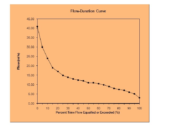
Flow Mass Curve Total flow volume from a certain initial time t = 0 up to time t can be computed as, In practice, the total volume is computed as, where Qi = the average discharge in time interval (month, year) ti. Flow mass curve is a plot of the cumulative runoff from the hydrograph against time. The time scale is the same as for the hydrograph and may be in days, months or years. The volume ordinate may be in m 3 -days, m 3 -months, m 3 years, etc. The slope of the mass curve is the rate of discharge.

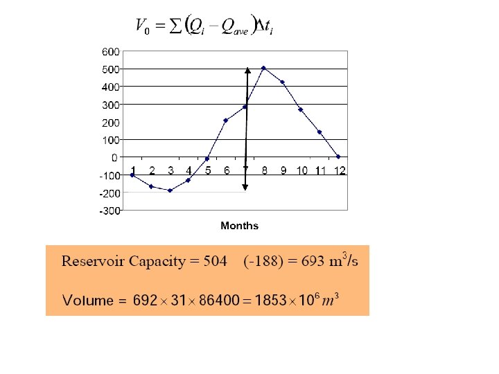
The ordinates of the flow mass curve increase continuously in time. The sum of the differences between the inflow and the yield (average flow) are drawn; Reservoir capacity is then, the vertical distance between the highest and lowest points of the curve. V 0 Fig. Flow mass curve derived using the differences of the discharges from the yield.

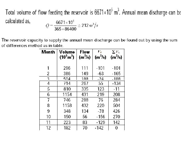
Example Monthly flow volumes feeding a reservoir are given in the table. Determine the storage capacity required to supply the mean annual flow volume yield.

Turbine selection criteria • Generally the selection shall be based on: – Available head – Available discharge – Power demand fluctuation – Cost • For small head, the discharge requirement is high, requiring bigger turbines; thus costly.

• The choice of a suitable hydraulic prime-mover depends upon various considerations for the given head and discharge at a particular site of the power plant. • The type of the turbine can be determined if the head available, power to be developed and speed at which it has to run are known to the engineer beforehand. The following factors have the bearing on the selection of the right type of hydraulic turbine: – Rotational Speed; – Specific Speed; – Maximum Efficiency;

Introduction to Small hydropower system design using RETScreen Small hydro systems harness the power of falling water to provide electricity for: §Central-grids; §Isolated-grids; and §Remote power supply Small hydro projects can be integrated on to central or isolated grids. A central grid is one that covers a vast geographical area, with many generators and millions of consumers. An isolated grid is a smaller network of generation and distribution facilities, not interconnected with the central grid, that supplies electricity to a limited area.

Ø Small hydro systems are used to power remote communities, mines, and camps that are not served by the grid. Ø Very small hydro systems can even be used to provide electricity to individual off-grid homes. Ø Small hydro systems can generate large amounts of electricity with very low operating costs. Ø The major costs of a small hydro project arise from expenses in construction and equipment purchase. Once the development is in place, the project can provide electricity with modest operation and maintenance expenditures for 50 years or longer.

“Small” is not universally defined. Ø Small hydro projects include mini and micro hydro projects. Ø Small hydro projects can be classified according to a number of criteria, including the rated power output of the project, the flow rate, and the diameter of the runner, that is, the spinning wheel within the turbine. Ø The problem with using the power capacity is that a very small high head project can generate with a small flow the same power as an enormous low head project requiring a huge flow. Ø Using the runner diameter, which is closely related to the flow through the turbine, is a more logical choice.

Ø Micro hydro refers to projects using turbines with a runner diameter less than 0. 3 m; this corresponds to a max. flow rate of 0. 4 m 3/s. Ø Mini hydro projects have turbines with runners 0. 3 to 0. 8 m in diameter and have max. flow rates of 0. 4 m 3/s to 12. 8 m 3/s. Ø This upper limit is the flow permitted by four turbines operating in parallel, each operating with 0. 8 m runner diameter. • The use of more than four mini turbines is not economical compared with a single larger turbine. So projects with maximum flow rates above 12. 8 m 3/s make use of turbines with runner diameters greater than 0. 8 m and are therefore not considered mini hydro projects. • They are simply known as small hydro projects.

Small Hydro Energy Calculations Ø Based on the hygrograph of the site the flow duration and load duration curves can be generated. Ø The following energy related quantities, for a small hydropower are determined: § Energy demand Ed ; Annual Energy Demand ED ; § Available power P; § Available renewable energy EAvail ; § Energy delivered Edlvd; and § Daily and Annually delivered energy.

ØSmall Hydro Energy calculation determines the energy delivered by a hydro project over the period of a year. Ø Data used for this calculation are the head, various component efficiencies, a flow duration curve representative of the flow over the year and, for isolated grids, a load duration curve. Ø Flow duration curve is a plot that shows the percentage of time that flow in a stream is likely to equal or exceed some specified value. Ø Load duration curve describes annual variation in the load for an isolated grid; Like flow duration curve, it is expressed in terms of the load that is exceeded for a specified fraction of the year.

Ø Step 1 Calculation of turbine efficiency as a function of flow rate: Ø Available empirical relations are used to calculate the turbine efficiency or Ø The turbine efficiency can also be assumed as a function of flow. Step 2: Calculation of the plant capacity: Ø The plant power output can be determined from empirical equation as a function of flow. Ø The power output is the product of the mass flow rate, the acceleration due to gravity, the head, the turbine efficiency at the given flow rate, the generator efficiency and the transmission system efficiency, all reduced by the parasitic losses.

Ø This calculation uses the net head; that is, the difference in elevation between the surface of the water above the intake and the turbine minus hydraulic losses caused by resistance to water flow in the passages between the intake and the turbine. Ø The plant capacity is the power output, as found from this equation, with the flow rate set to the design flow rate. Step 3: Calculation of the power duration curve: Ø The power duration curve is constructed from the flow duration curve: for each point on the flow duration curve, the corresponding plant output is calculated from the equation for power as a function of flow. Ø When the available flow exceeds the design flow, the design flow is used as the independent variable in the equation.

Step 4: Calculation of available energy: Ø The available energy is calculated by integrating the area underneath the power duration curve. Step 5: Calculation of the energy delivered: Ø Central grids can absorb all the energy produced by the plant, so for them, the energy delivered is equal to the available energy. Ø For isolated grid plants, output of the plant in excess of the load is not used, so the power duration curve must be compared with the load duration curve to determine which is the limiting consideration.

Ø The power duration curve is divided into 20 segments, each representing the power output during 5% of the year. An example of a power duration curve is shown in Fig. below for a design flow of 3 m 3/s. Fig. Typical flow duration and power curves

Ø Then the area under the load duration curve that lies below this power level is used to determine the energy delivered during that 5% of the year. Ø The annual energy delivered is the sum of the energy delivered in all of the 20 segments. Fig. Typical flow duration curve and data

Energy Production Ø Demand – refers to integrated values. Ø Daily energy demand – area under load-duration curve over a day. Ø A simple trapezoidal integration formula is used. Ø The daily energy demand Dd [k. Wh] is calculated from: The annual energy demand D is obtained by multiplying the daily demand by the number of days in a year, 365:

Ø Average load factor – the ratio of the average daily load to the peak load is obtained from: Available Power as a Function of Flow Actual power P available from a small hydropower plant for a given flow rate Q is given by the following equation, in which the flow-dependent hydraulic losses and tailrace reduction are taken into account: where is the density of water, g the acceleration of gravity, Hg the gross head, hhydr and htail are respectively the hydraulic losses and tailrace effect associated with the flow, t is the turbine efficiency at flow Q, g is the generator efficiency, htrans the transformer losses, and hpara the parasitic electricity losses

Plant Capacity Ø The plant capacity Pdes of a hydropower plant as a function of design flow Qdes can be estimated from:

Ø Available renewable energy is determined by calculating the area under the power curve, assuming a straight line between adjacent calculated power output values. Ø Given that the flow-duration curve represents an annual cycle, each 5% interval on the curve is equivalent to 5% of 8760 hours (number of hours per year). Ø The annual available energy E avail is determined from: where: hdt is the annual downtime losses ( = 2 to 7%)

Energy Delivered to Central Grid: Ø For central-grid applications, it is assumed that the grid is able to absorb all the energy produced by the small hydro power plant. Ø All the renewable energy available, therefore, will be delivered to the central-grid and the renewable energy delivered, Edlvd, is: Energy Delivered to Isolated Grid and Off-Grid: The portion of energy that can be delivered by the small hydro plant is determined as the area that is under both the load duration curve and the horizontal line representing the available plant power output.

Fig. Example : Daily Renewable Energy Delivered

Friction head losses in closed pipe Where: S is the hydraulic gradient or head loss by linear meter (hf/L). Q is the channel discharge (m 3/s) n is the Manning roughness coefficient

RETScreen Small Hydro Project Model ® • World-wide analysis of energy production, life-cycle costs and greenhouse gas emissions reductions – Central-grid, isolated-grid and off-grid – Single turbine micro hydro to multi-turbine small hydro – “Formula” costing method • Currently not covered: – Seasonal variations in isolated-grid load – Variations in head in storage projects (user must supply average value) © Minister of Natural Resources Canada 2001 – 2004.

RETScreen Small Hydro ® Energy Calculation See e-Textbook Clean Energy Project Analysis: RETScreen® Engineering and Cases Small Hydro Project Analysis Chapter © Minister of Natural Resources Canada 2001 – 2004.

Example Validation of the RETScreen® Small Hydro Project Model • Turbine efficiency – Compared with manufacturer’s data for an installed 7 MW GEC Alsthom Francis turbine © Minister of Natural Resources Canada 2001 – 2004.

Conclusions • Small hydro projects (up to 50 MW) can provide electricity for central or isolated-grids and for remote power supplies • Run-of-river projects: – Lower cost & lower environmental impacts – But need back-up power on isolated grid • Initial costs high and 75% site specific • RETScreen® estimates capacity, firm capacity, output and costs based on site characteristics such as flow-duration curve and head • RETScreen® can provide significant preliminary feasibility study cost savings © Minister of Natural Resources Canada 2001 – 2004.