Chapter 5 Who gains and who loses from

Chapter 5 Who gains and who loses from trade? Also will look at Appendix B. Link to syllabus

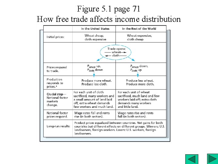
Figure 5. 1 page 71 How free trade affects income distribution

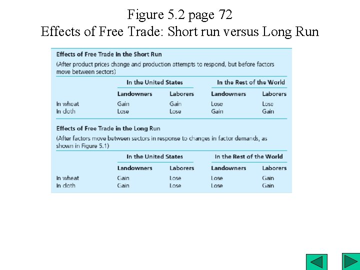
Figure 5. 2 page 72 Effects of Free Trade: Short run versus Long Run

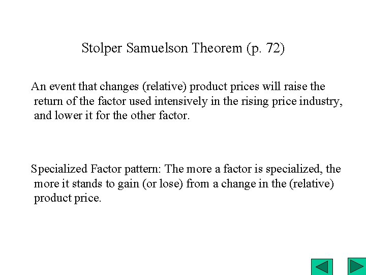
Stolper Samuelson Theorem (p. 72) An event that changes (relative) product prices will raise the return of the factor used intensively in the rising price industry, and lower it for the other factor. Specialized Factor pattern: The more a factor is specialized, the more it stands to gain (or lose) from a change in the (relative) product price.

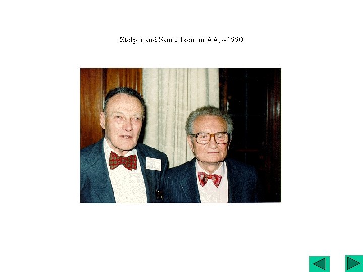
Stolper and Samuelson, in AA, ~1990

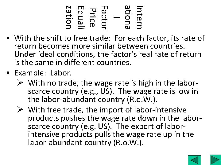
Intern ationa l Factor Price Equali zation • With the shift to free trade: For each factor, its rate of return becomes more similar between countries. Under ideal conditions, the factor’s real rate of return is the same in different countries. • Example: Labor. Ø With no trade, the wage rate is high in the laborscarce country (e. g. , US). The wage rate is low in the labor-abundant country (R. o. W. ). Ø With free trade, the import of labor-intensive products pushes the wage rate down in the laborscarce country (e. g. US). The export of laborintensive products pulls the wage rate up in the labor-abundant country (R. o. W. ).

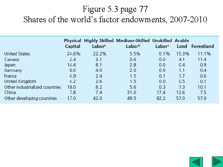
Figure 5. 3 page 77 Shares of the world’s factor endowments, 2007 -2010

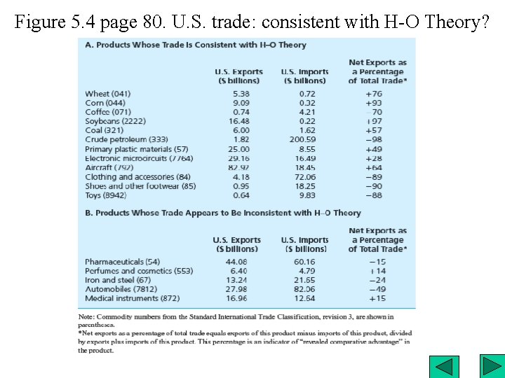
Figure 5. 4 page 80. U. S. trade: consistent with H-O Theory?

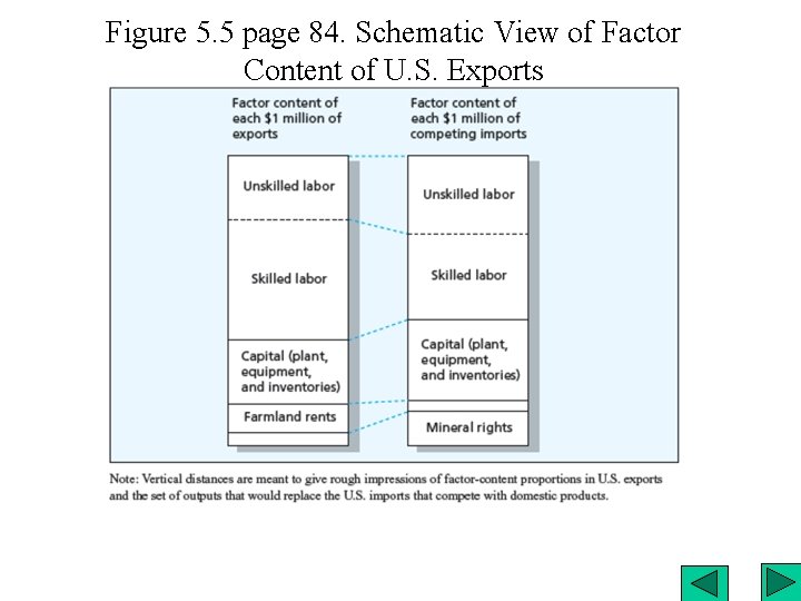
Figure 5. 5 page 84. Schematic View of Factor Content of U. S. Exports

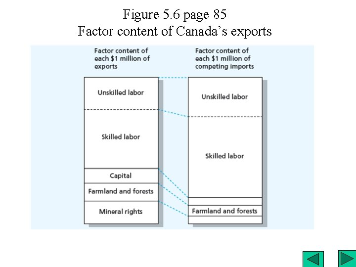
Figure 5. 6 page 85 Factor content of Canada’s exports

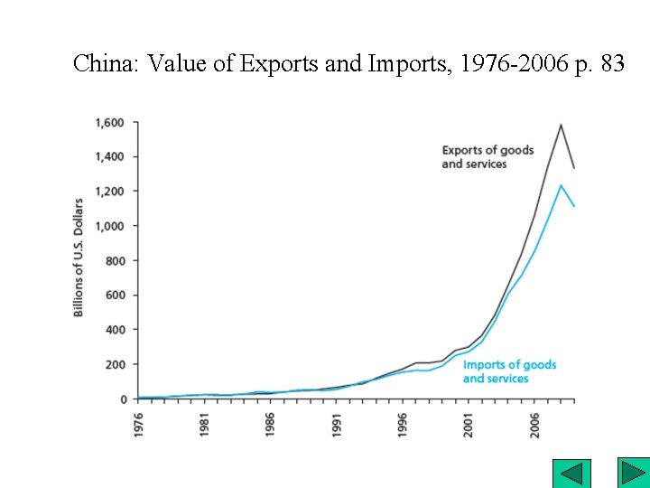
China: Value of Exports and Imports, 1976 -2006 p. 83

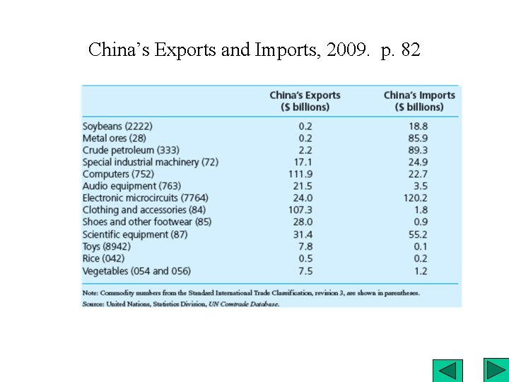
China’s Exports and Imports, 2009. p. 82

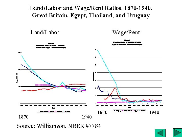
Land/Labor and Wage/Rent Ratios, 1870 -1940. Great Britain, Egypt, Thailand, and Uruguay Land/Labor 1870 Wage/Rent 1940 1870 Source: Williamson, NBER #7784 1940

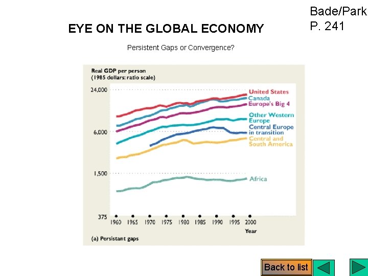
EYE ON THE GLOBAL ECONOMY Persistent Gaps or Convergence? Back to list Bade/Parki P. 241

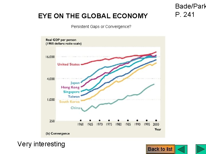
EYE ON THE GLOBAL ECONOMY Persistent Gaps or Convergence? Very interesting Back to list Bade/Park P. 241

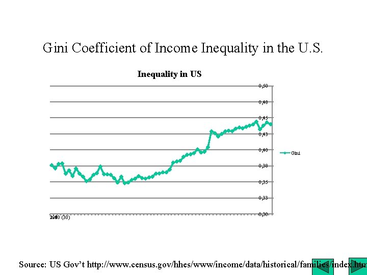
Gini Coefficient of Income Inequality in the U. S. Inequality in US 0, 50 0, 48 0, 45 0, 43 0, 40 Gini 0, 38 0, 35 0, 33 2010 1950 1960 1970 1980 1990 2000 (30) 0, 30 Source: US Gov’t http: //www. census. gov/hhes/www/income/data/historical/families/index. htm

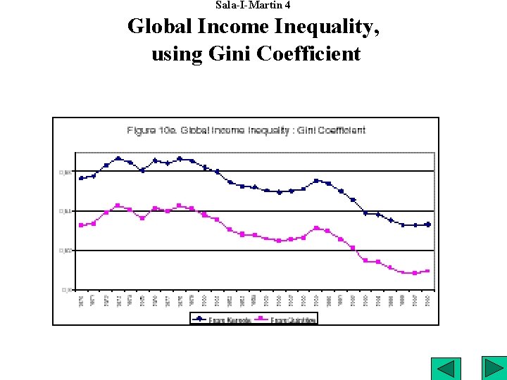
Sala-I-Martin 4 Global Income Inequality, using Gini Coefficient

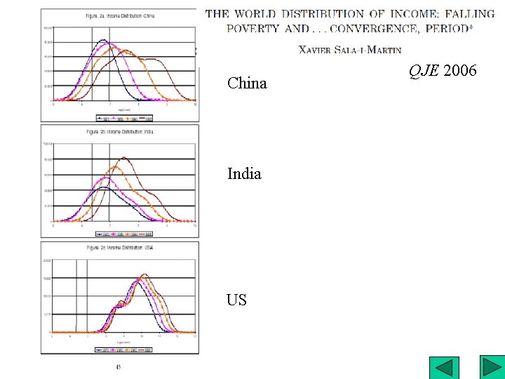
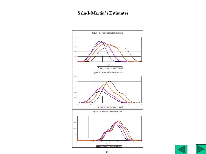
Sala-I-Martin’s Estimates China India US QJE 2006

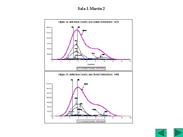
Sala-I-Martin 2

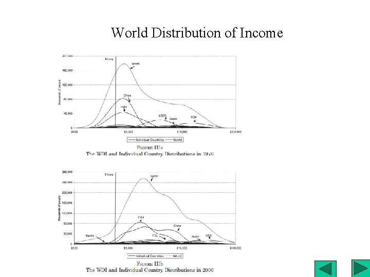
World Distribution of Income

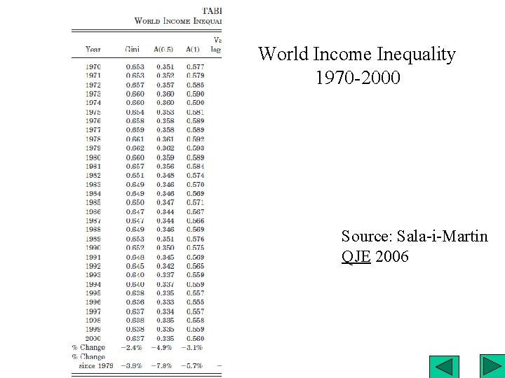
World Income Inequality 1970 -2000 Source: Sala-i-Martin QJE 2006

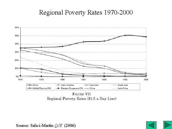
Regional Poverty Rates 1970 -2000 Source: Sala-i-Martin QJE (2006)

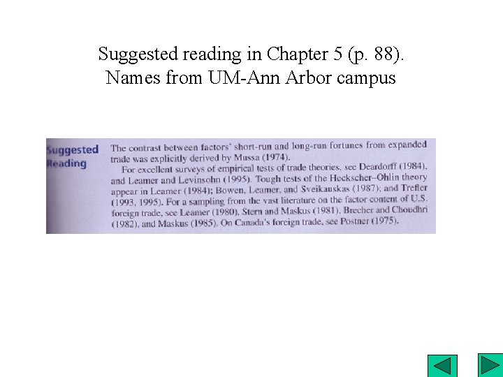
Suggested reading in Chapter 5 (p. 88). Names from UM-Ann Arbor campus

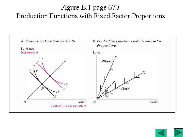
Figure B. 1 page 670 Production Functions with Fixed Factor Proportions

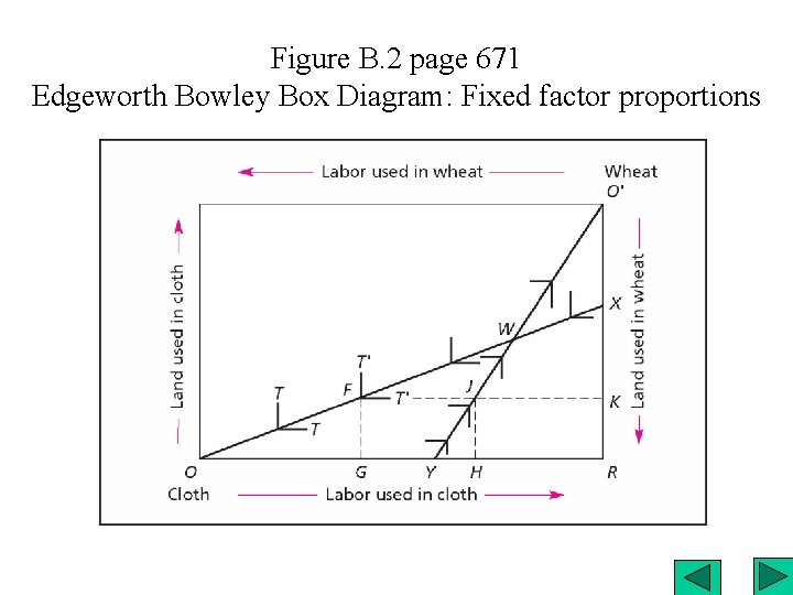
Figure B. 2 page 671 Edgeworth Bowley Box Diagram: Fixed factor proportions

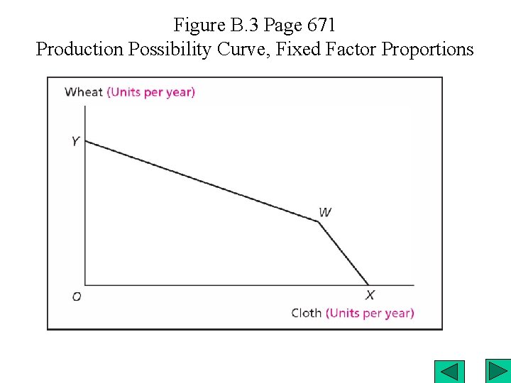
Figure B. 3 Page 671 Production Possibility Curve, Fixed Factor Proportions

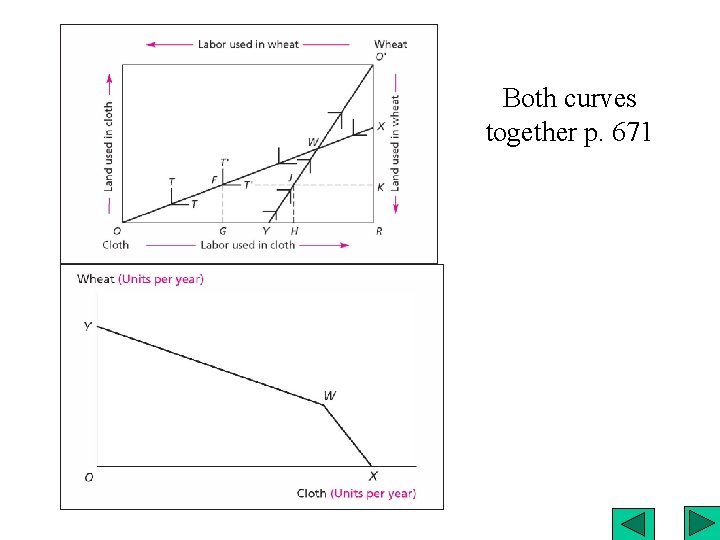
Both curves together p. 671

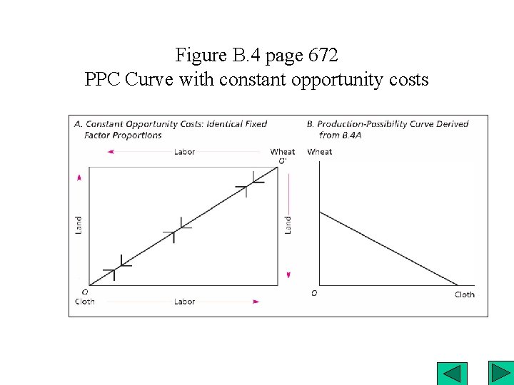
Figure B. 4 page 672 PPC Curve with constant opportunity costs

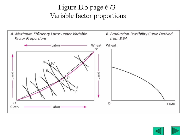
Figure B. 5 page 673 Variable factor proportions

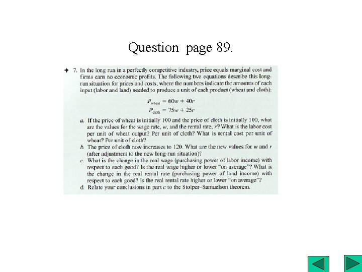
Question page 89.

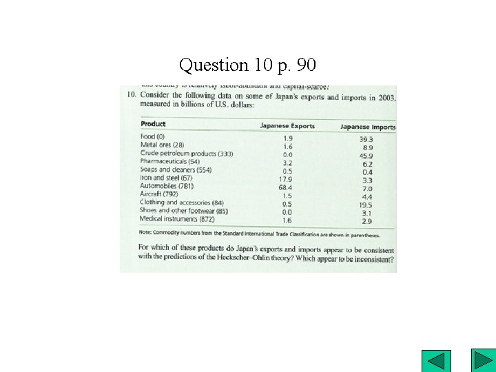
Question 10 p. 90

Sala-I-Martin’s Estimates

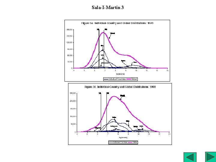
Sala-I-Martin 3