CHAPTER 3 The Data Warehouse and Design BEGINNING

CHAPTER: -3 The Data Warehouse and Design

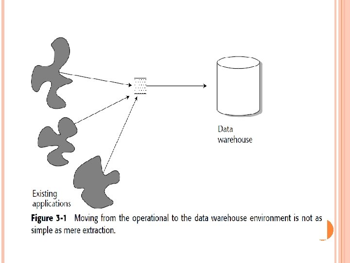
BEGINNING WITH OPERATIONAL DATA Design begins with the considerations of placing data in the data warehouse. There are many considerations to be made concerning the placement of data into the data warehouse from the operational environment.

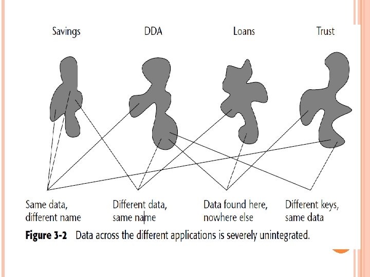
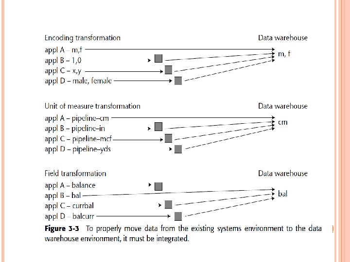
Figure 3 -1 shows a simplification of how data is transferred from the existing legacy systems environment to the data warehouse. We see here that multiple applications contribute their data to the data warehouse. Figure 3 -1 is overly simplistic for many reasons. Most importantly, it does not take into account that the data in the operational environment is unintegrated. Figure 3 -2 shows the lack of integration in a typical existing systems environment. Pulling the data into the data warehouse without integrating it is a grave mistake.

Three types of loads are made into the data warehouse from the operational environment: Archival data Data currently contained in the operational environment Ongoing changes to the data warehouse environment from the changes (updates) that have occurred in the operational environment since the last refresh

First, it often is not done at all. Organizations find the use of old data not cost-effective in many environments. Second, even when archival data is loaded, it is a onetime-only event.

FIVE COMMON TECHNIQUES Five common techniques are used to limit the amount of operational data scanned at the point of refreshing the data warehouse, as shown in Figure 3 -4. The first technique is to scan data that has been time stamped in the operational environment. When an application stamps the time of the last change or update on a record, the data warehouse scan run quite efficiently because data with a date other than that applicable does not have to be touched.

The second technique to limiting the data to be scanned is to scan a delta file. A delta file contains only the changes made to an application as a result of the transactions that have run through the operational environment. With a delta file, the scan process is very efficient because data that is not a candidate for scanning is never touched. The third technique is to scan a log file or an audit file created as a by-product of transaction processing. A log file contains essentially the same data as a delta file. However, there are some major differences. Many times, computer operations protects the log files because they are needed in the recovery process.

The fourth technique for managing the amount of data scanned is to modify application code. The last option (in most respects, a hideous one from a resource-utilization perspective, mentioned primarily to convince people that there must be a better way) is rubbing a “before” and an “after” image of the operational file together. In this option, a snapshot of a database is taken at the moment of extraction. When another extraction is performed, another snapshot is taken. The two snapshots are serially compared to each other to determine the activity that has transpired. This approach is cumbersome and complex, and it requires an inordinate amount of resources.

Figure 3 -4 How do you know what source data to scan? Do you scan every record every day? Every week?

PROCESS AND DATA MODELS AND THE ARCHITECTED ENVIRONMENT The process model applies only to the operational environment. The data model applies to both the operational environment and the data warehouse environment.

Figure 3 -7 How the different types of models apply to the architected environment.

A process model typically consists of the following (in whole or in part): ■ Functional decomposition ■ Context-level zero diagram ■ Data flow diagram ■ Structure chart ■ State transition diagram ■ HIPO chart ■ Pseudo code There are many contexts and environments in which a process model is invaluable—for example, when building the data mart.

THE DATA WAREHOUSE AND DATA MODELS FIGURE 3 -8 HOW THE DIFFERENT LEVELS OF MODELING RELATE.

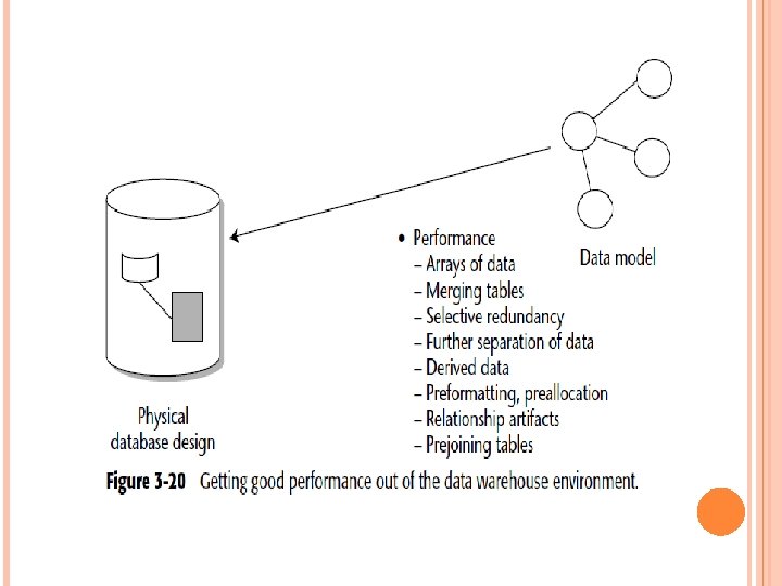
Operational data model equals corporate data model Performance factors are added prior to database design Remove pure operational data Add element of time to key Add derived data where appropriate Create artifacts of relationships

THE DATA WAREHOUSE AND DATA MODELS As shown in Figure 3 -8, the data model is applicable to both the existing systems environment and the data warehouse environment. Here, an overall corporate data model has been constructed with no regard for a distinction between existing operational systems and the data warehouse.

Stability analysis involves grouping attributes of data together based on their propensity for change. Figure 3 -9 illustrates stability analysis for the manufacturing environment. Three tables are created from one large generalpurpose table based on the stability requirements of the data contained in the tables.

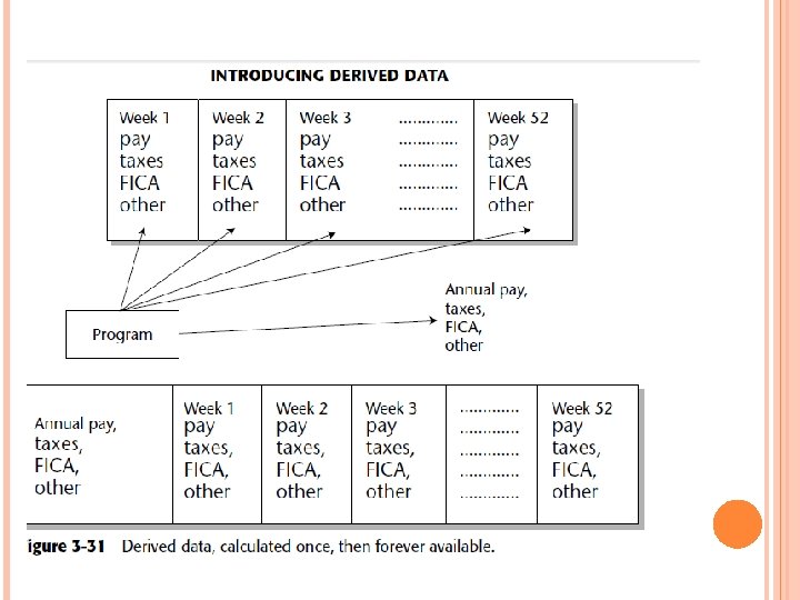
However, a fair number of changes are made to the corporate data model as it is applied to the data warehouse. First, data that is used purely in the operational environment is removed. Next, the key structures of the corporate data model are enhanced with an element of time if they don’t already have an element of time. Derived data is added to the corporate data model where the derived data is publicly used and calculated once, not repeatedly.

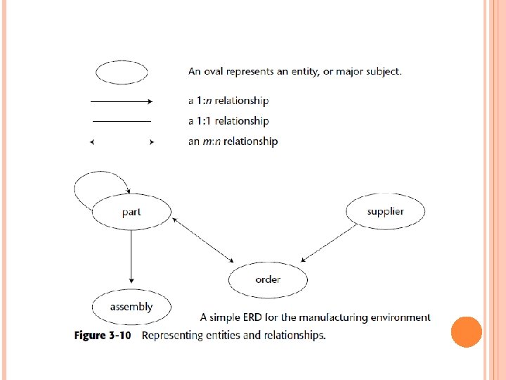
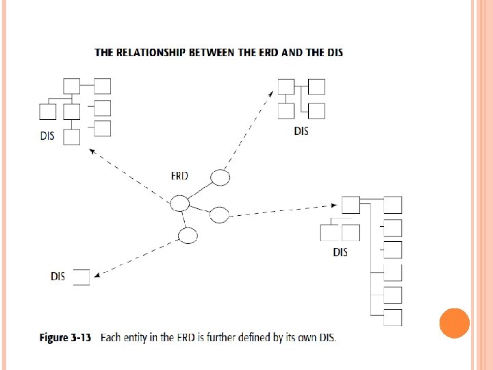
THE DATA WAREHOUSE DATA MODEL There are three levels of data modeling: high-level modeling (called the entity relationship diagram, or ERD), midlevel modeling (called the data item set, or DIS), and low-level modeling (called the physical model). The high level of modeling features entities and relationships, as shown in Figure 3 -10. The name of the entity is surrounded by an oval. Relationships among entities are depicted with arrows. The direction and number of the arrowheads indicate the cardinality of the relationship, and only direct relationships are indicated.

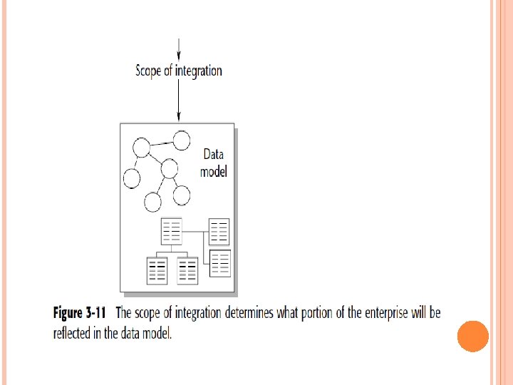
Figure 3 -11. The scope of integration defines the boundaries of the data model and must be defined before the modeling process commences. The scope is agreed on by the modeler, the management, and the ultimate user of the system. If the scope is not predetermined, there is the great chance that the modeling process will continue forever.

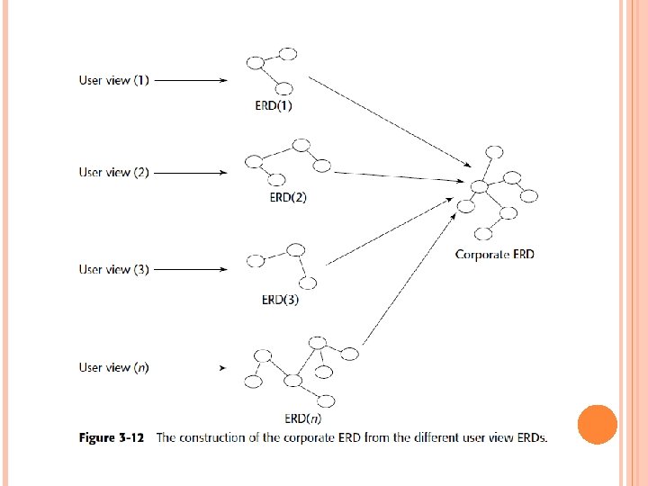
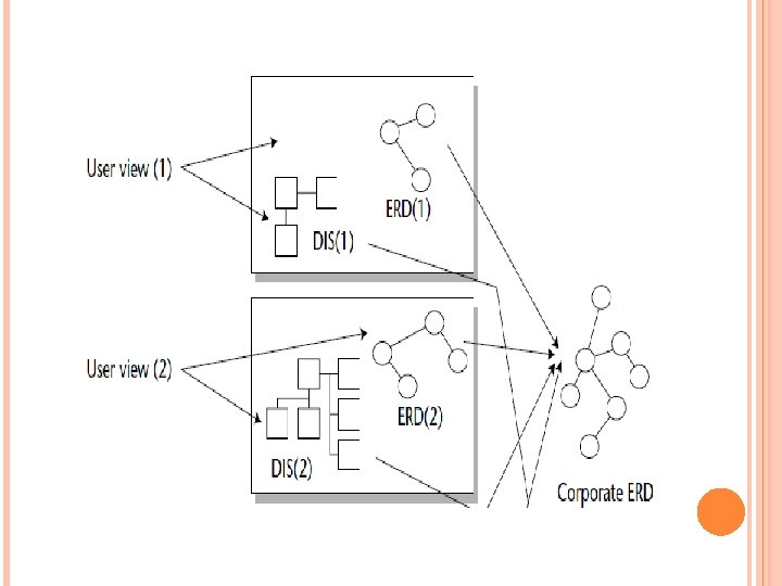
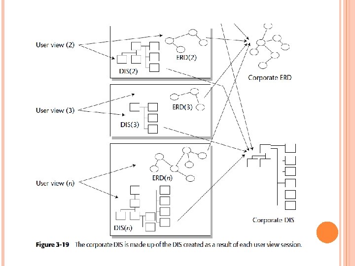
As shown in Figure 3 -12, the corporate ERD is a composite of many individual ERDs that reflect the different views of people across the corporation. Separate high-level data models have been created for different communities within the corporation. Collectively, they make up the corporate ERD. The ERDs representing the known requirements of the DSS community are created by means of user view sessions or Joint Application Design (JAD) sessions,

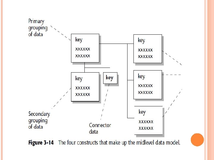
THE MIDLEVEL DATA MODEL The high-level data model has identified four entities, or major subject areas. Each area is subsequently developed into its own midlevel model. As shown in Figure 3 -14, four basic constructs are found at the midlevel model. A primary grouping of data The primary grouping exists once, and only once, for each major subject area. It holds attributes that exist only once for each major subject area.

A secondary grouping of data The secondary grouping holds data attributes that can exist multiple times for each major subject area. This grouping is indicated by a line emanating downward from the primary grouping of data. A connector—This signifies the relationships of data between major subject areas. The connector relates data from one grouping to another.

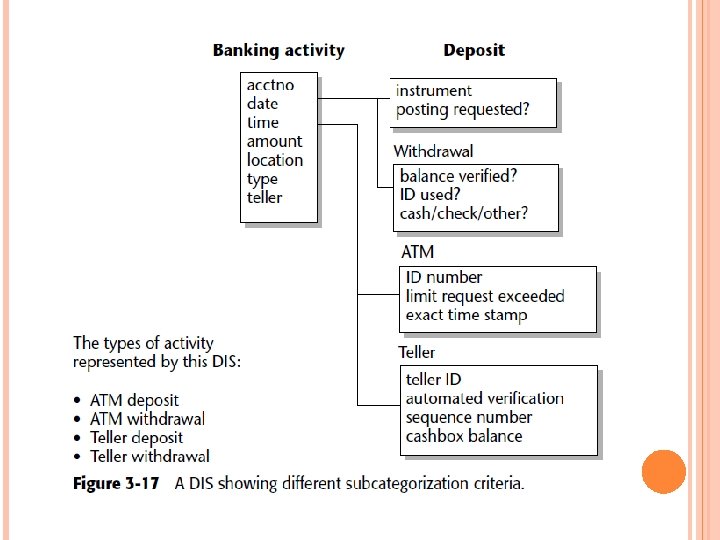
“Type of” data: This data is indicated by a line leading to the right of a grouping of data. The grouping of data to the left is the supertype. These four data modeling constructs are used to identify the attributes of data in a data model and the relationship among those attributes.

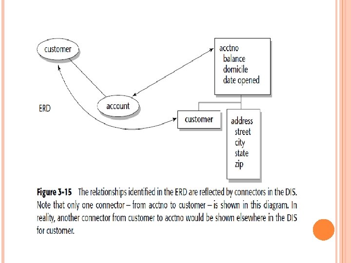
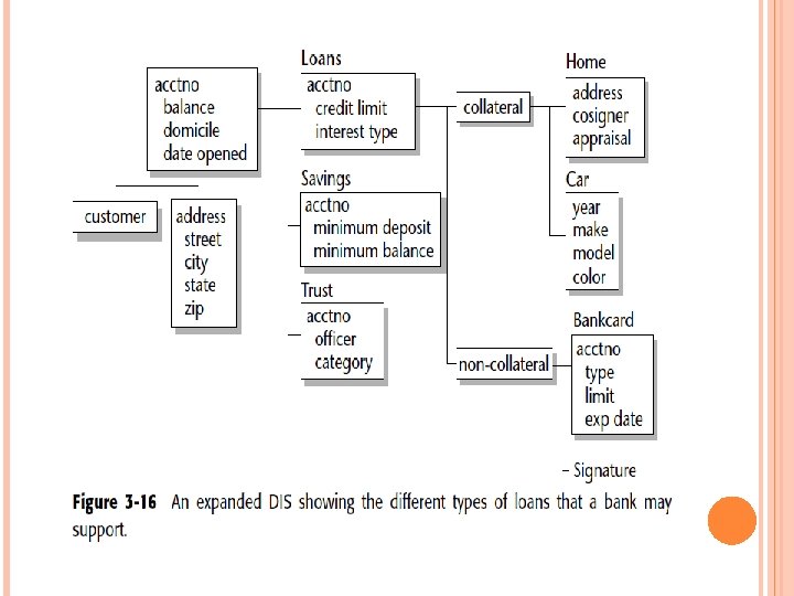
At the ERD, a relationship between customer and account has been identified. At the DIS level for account, there exists a connector beneath account. This indicates that an account may have multiple customers attached to it. Not shown is the corresponding relationship beneath the customer in the customer. DIS. Figure 3 -16 shows what a full-blown DIS might look like, where a DIS exists for an account for a financial institution

THE PHYSICAL DATA MODEL The physical data model is created from the midlevel data model merely by extending the midlevel data model to include keys and physical characteristics of the model. At this point, the physical data model looks like a series of tables, sometimes called relational tables.

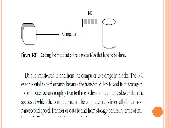
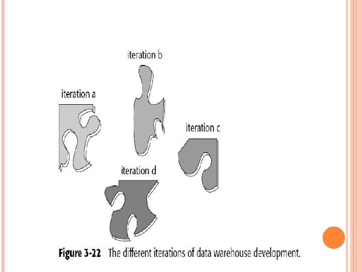
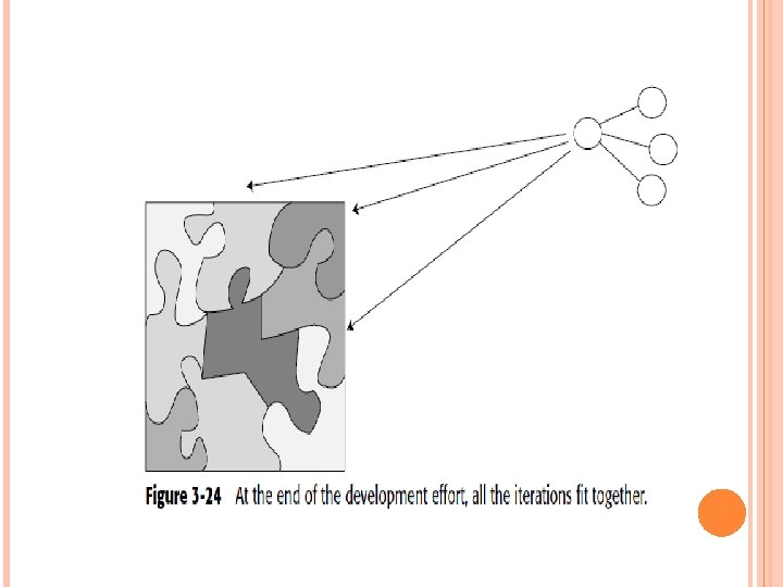
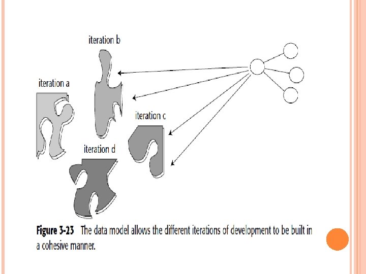
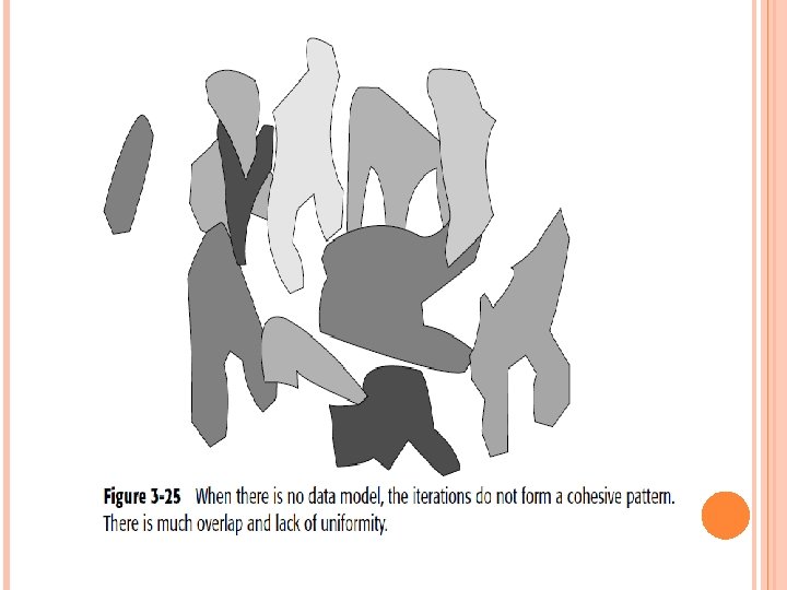
THE DATA MODEL AND ITERATIVE DEVELOPMENT This means that first one part of the data warehouse is built, and then another part of the data warehouses built, and so forth. The following are some of the many reasons why iterative development is important: The industry track record of success strongly suggests it. The end user is unable to articulate many requirements until the first iteration is done. Computer I/O Management will not make a full commitment until at least a few actual results are tangible and obvious. Visible results must be seen quickly.

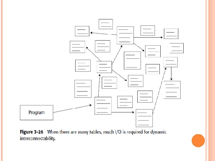
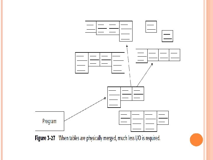
NORMALIZATION AND DENORMALIZATION The output of the data model process is a series of tables, each of which contains keys and attributes. In Figure 3 -26, a program goes into execution. First, one table is accessed, then another. To execute successfully, the program must jump around many tables. Each time the program jumps from one table to the next, I/O is consumed, in terms of both accessing the data and accessing the index to find the data.

If only one or two programs had to pay the price of I/O, there would be no problem. But when all programs must pay a stiff price for I/O, performance in general suffers, and that is precisely what happens when many small tables, each containing a limited amount of data, are created as a physical design.

Merging tables is only one design technique that can save I/O. Another very useful technique is creating an array of data. In Figure 3 -28, data is normalized so that each occurrence of a sequence of data resides in a different physical location. Retrieving each occurrence, n, n + 1, n + 2, . . . , requires a physical I/O to get the data.

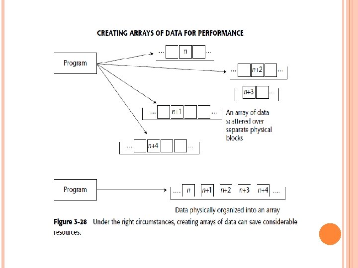
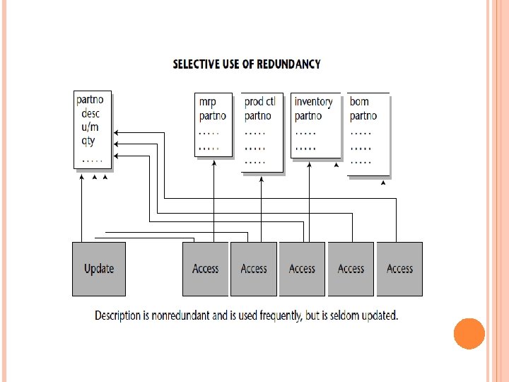
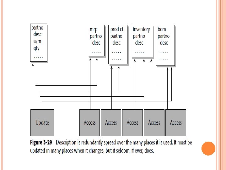
where the data is accessed in sequence, where it is created and/or updated in a statistically wellbehaved sequence, and so forth, does creating an array pay off. Another important physical design technique that is especially relevant to the data warehouse environment is the deliberate introduction of redundant data. Figure 3 -29 shows an example where the deliberate introduction of redundant data pays a big dividend. In the top of Figure 3 -29, the field-description (desc) —is normalized and exists nonredundantly

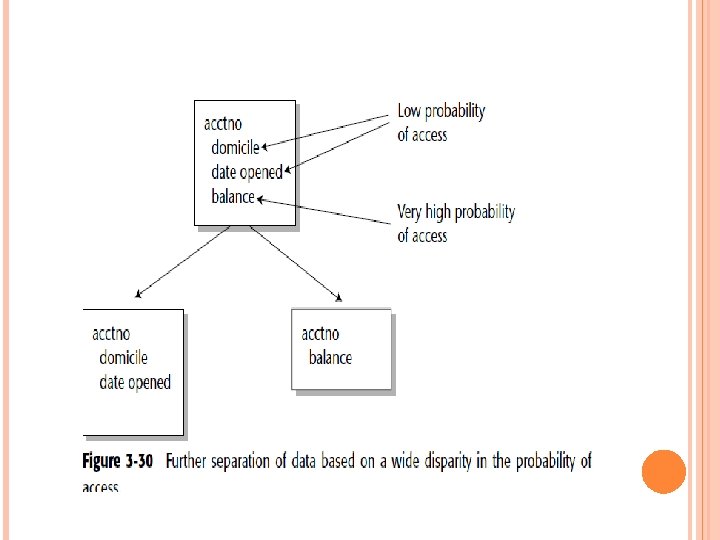
In the bottom of Figure 3 -29, the data element “description” (desc) has been deliberately placed in the many tables where it is likely to be used. Another useful technique is the further separation of data when there is a wide disparity in the probability of access. Figure 3 -30 shows such a case.

One of the most innovative techniques in building a data warehouse is what can be termed a creative index, or a creative profile. Figure 3 -32 shows an example of a creative index. This type of creative index is created as data is passed from the operational environment to the data warehouse environment.

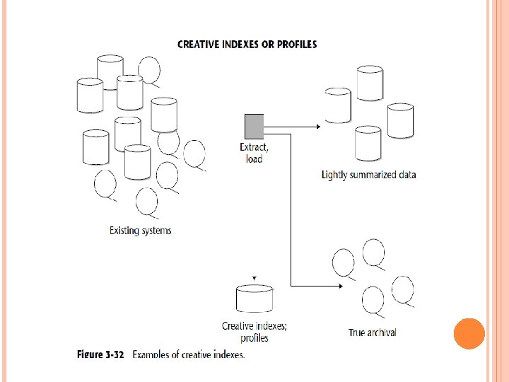
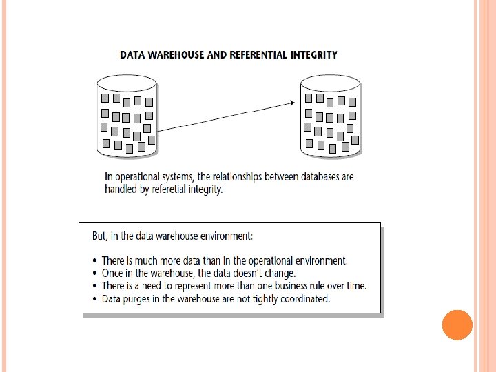
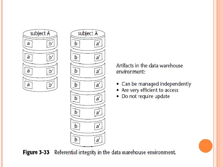
The creative index does a profile on items of interest to the end user, such as the largest purchases, the most inactive accounts, the latest shipments, and so on. A final technique that the data warehouse designer should keep in mind is the management of referential integrity. Figure 3 -33 shows that referential integrity appears as “artifacts” of relationships in the data warehouse environment.

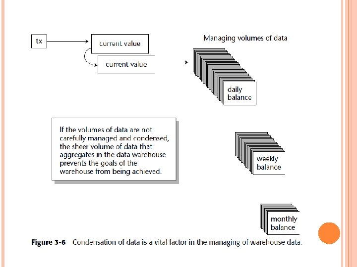
METADATA An important component of the data warehouse environment is metadata (or data about data), which has been a part of the information processing milieu for as long as there have been programs and data. Metadata then acts like an index to the contents of the data warehouse. It consist above the warehouse and keeps track of what is where in the warehouse. Typically, items the metadata store tracks are as follows:

Structure of data as known to the programmer Structure of data as known to the DSS analyst Source data feeding the data warehouse Transformation of data as it passes into the data warehouse Data model Relationship between the data model and the data warehouse History of extracts

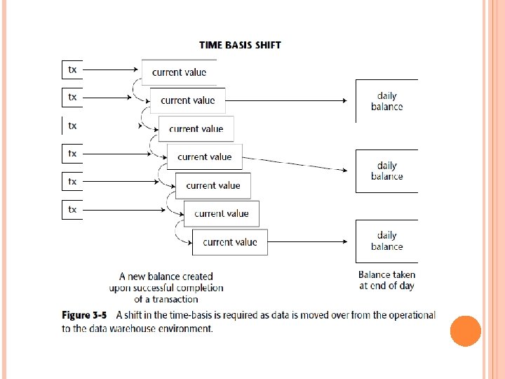
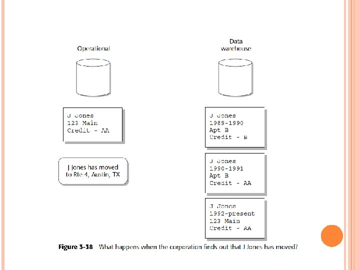
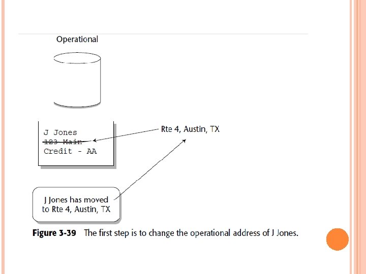
Cyclicity of Data — The Wrinkle of Time One of the intriguing issues of data warehouse design is the cyclicity of data, orthe length of time a change of data in the operational environment takes to be reflected in the data warehouse. Figure 3 -39 shows that as soon as that change is discovered, it isreflected in the operational environment as quickly as possible.