Data Warehouse Tuning Datawarehouse Tuning Aggregate strategic targeting

Data Warehouse Tuning

Datawarehouse Tuning • Aggregate (strategic) targeting: – Aggregates flow up from a wide selection of data, and then – Targeted decisions flow down • Examples: – Riding the wave of clothing fads – Tracking delays for frequent-flyer customers 7 - Datawarehouse 2

Data Warehouse Workload • Broad – Aggregate queries over ranges of values, e. g. , find the total sales by region and quarter. • Deep – Queries that require precise individualized information, e. g. , which frequent flyers have been delayed several times in the last month? • Dynamic (vs. Static) – Queries that require up-to-date information, e. g. which nodes have the highest traffic now? 7 - Datawarehouse 3

Tuning Knobs • Indexes • Materialized views • Approximation 7 - Datawarehouse 4

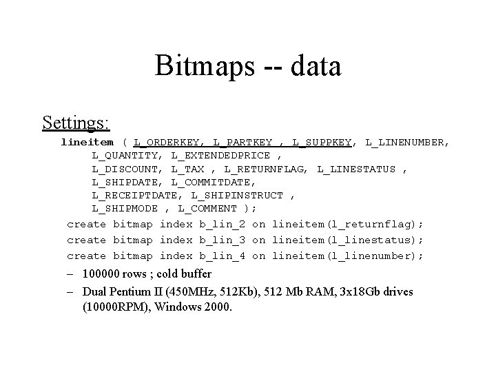
Bitmaps -- data Settings: lineitem ( L_ORDERKEY, L_PARTKEY , L_SUPPKEY, L_LINENUMBER, L_QUANTITY, L_EXTENDEDPRICE , L_DISCOUNT, L_TAX , L_RETURNFLAG, L_LINESTATUS , L_SHIPDATE, L_COMMITDATE, L_RECEIPTDATE, L_SHIPINSTRUCT , L_SHIPMODE , L_COMMENT ); create bitmap index b_lin_2 on lineitem(l_returnflag); create bitmap index b_lin_3 on lineitem(l_linestatus); create bitmap index b_lin_4 on lineitem(l_linenumber); – 100000 rows ; cold buffer – Dual Pentium II (450 MHz, 512 Kb), 512 Mb RAM, 3 x 18 Gb drives (10000 RPM), Windows 2000.

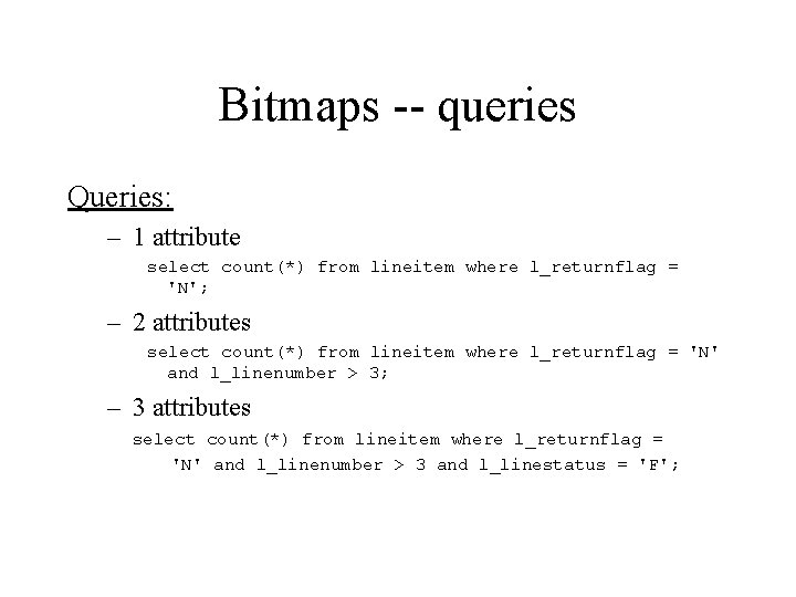
Bitmaps -- queries Queries: – 1 attribute select count(*) from lineitem where l_returnflag = 'N'; – 2 attributes select count(*) from lineitem where l_returnflag = 'N' and l_linenumber > 3; – 3 attributes select count(*) from lineitem where l_returnflag = 'N' and l_linenumber > 3 and l_linestatus = 'F';

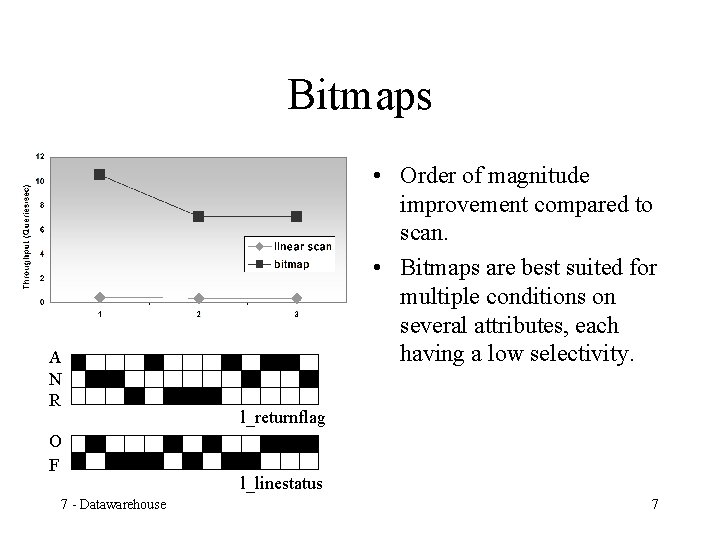
Bitmaps A N R O F 7 - Datawarehouse • Order of magnitude improvement compared to scan. • Bitmaps are best suited for multiple conditions on several attributes, each having a low selectivity. l_returnflag l_linestatus 7

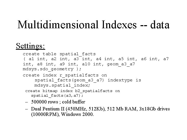
Multidimensional Indexes -- data Settings: create table spatial_facts ( a 1 int, a 2 int, a 3 int, a 4 int, a 5 int, a 6 int, a 7 int, a 8 int, a 9 int, a 10 int, geom_a 3_a 7 mdsys. sdo_geometry ); create index r_spatialfacts on spatial_facts(geom_a 3_a 7) indextype is mdsys. spatial_index; create bitmap index b 2_spatialfacts on spatial_facts(a 3, a 7); – 500000 rows ; cold buffer – Dual Pentium II (450 MHz, 512 Kb), 512 Mb RAM, 3 x 18 Gb drives (10000 RPM), Windows 2000.

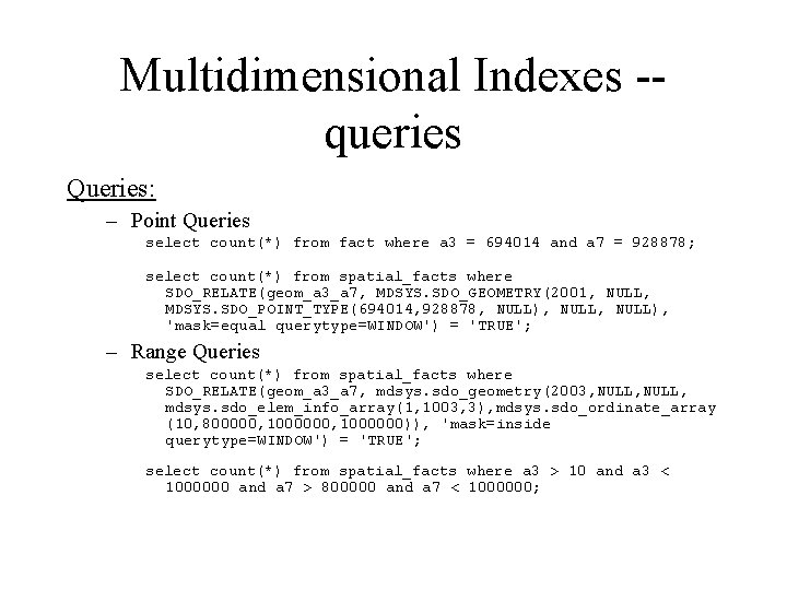
Multidimensional Indexes -queries Queries: – Point Queries select count(*) from fact where a 3 = 694014 and a 7 = 928878; select count(*) from spatial_facts where SDO_RELATE(geom_a 3_a 7, MDSYS. SDO_GEOMETRY(2001, NULL, MDSYS. SDO_POINT_TYPE(694014, 928878, NULL), 'mask=equal querytype=WINDOW') = 'TRUE'; – Range Queries select count(*) from spatial_facts where SDO_RELATE(geom_a 3_a 7, mdsys. sdo_geometry(2003, NULL, mdsys. sdo_elem_info_array(1, 1003, 3), mdsys. sdo_ordinate_array (10, 800000, 1000000)), 'mask=inside querytype=WINDOW') = 'TRUE'; select count(*) from spatial_facts where a 3 > 10 and a 3 < 1000000 and a 7 > 800000 and a 7 < 1000000;

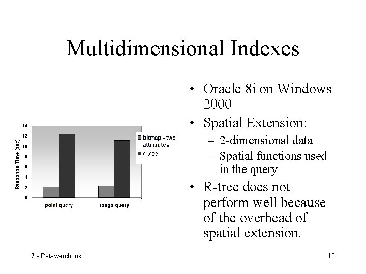
Multidimensional Indexes • Oracle 8 i on Windows 2000 • Spatial Extension: – 2 -dimensional data – Spatial functions used in the query • R-tree does not perform well because of the overhead of spatial extension. 7 - Datawarehouse 10

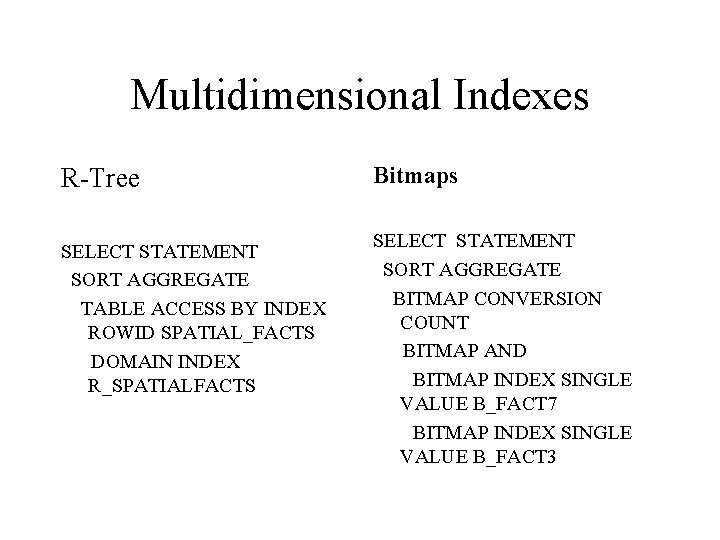
Multidimensional Indexes R-Tree SELECT STATEMENT SORT AGGREGATE TABLE ACCESS BY INDEX ROWID SPATIAL_FACTS DOMAIN INDEX R_SPATIALFACTS Bitmaps SELECT STATEMENT SORT AGGREGATE BITMAP CONVERSION COUNT BITMAP AND BITMAP INDEX SINGLE VALUE B_FACT 7 BITMAP INDEX SINGLE VALUE B_FACT 3

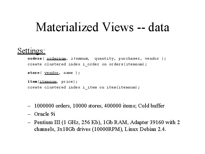
Materialized Views -- data Settings: orders( ordernum, itemnum, quantity, purchaser, vendor ); create clustered index i_order on orders(itemnum); store( vendor, name ); item(itemnum, price); create clustered index i_item on item(itemnum); – 1000000 orders, 10000 stores, 400000 items; Cold buffer – Oracle 9 i – Pentium III (1 GHz, 256 Kb), 1 Gb RAM, Adapter 39160 with 2 channels, 3 x 18 Gb drives (10000 RPM), Linux Debian 2. 4.

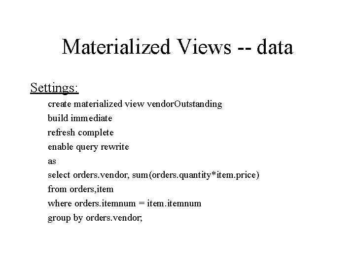
Materialized Views -- data Settings: create materialized view vendor. Outstanding build immediate refresh complete enable query rewrite as select orders. vendor, sum(orders. quantity*item. price) from orders, item where orders. itemnum = itemnum group by orders. vendor;

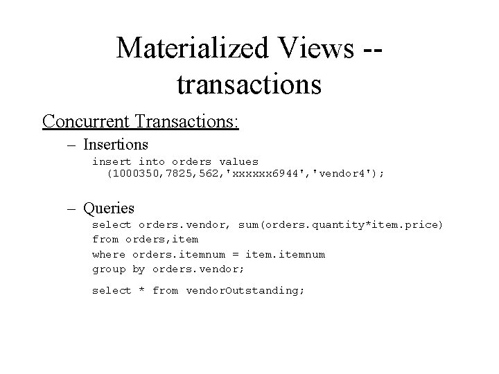
Materialized Views -transactions Concurrent Transactions: – Insertions insert into orders values (1000350, 7825, 562, 'xxxxxx 6944', 'vendor 4'); – Queries select orders. vendor, sum(orders. quantity*item. price) from orders, item where orders. itemnum = itemnum group by orders. vendor; select * from vendor. Outstanding;

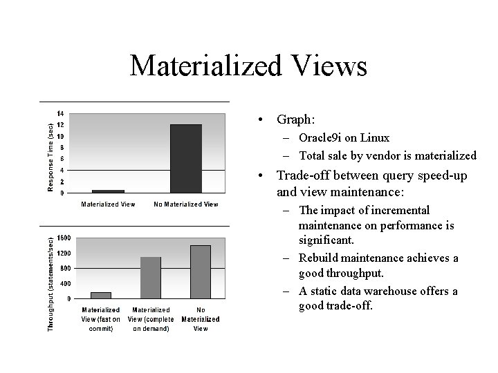
Materialized Views • Graph: – Oracle 9 i on Linux – Total sale by vendor is materialized • Trade-off between query speed-up and view maintenance: – The impact of incremental maintenance on performance is significant. – Rebuild maintenance achieves a good throughput. – A static data warehouse offers a good trade-off.

Materialized View Maintenance • Problem when large number of views to maintain. • The order in which views are maintained is important: – A view can be computed from an existing view instead of being recomputed from the base relations (total per region can be computed from total per nation). • • Let the views and base tables be nodes v_i Let there be an edge from v_1 to v_2 if it possible to compute the view v_2 from v_1. Associate the cost of computing v_2 from v_1 to this edge. Compute all pairs shortest path where the start nodes are the set of base tables. The result is an acyclic graph A. Take a topological sort of A and let that be the order of view construction.

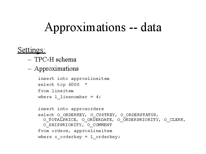
Approximations -- data Settings: – TPC-H schema – Approximations insert into approxlineitem select top 6000 * from lineitem where l_linenumber = 4; insert into approxorders select O_ORDERKEY, O_CUSTKEY, O_ORDERSTATUS, O_TOTALPRICE, O_ORDERDATE, O_ORDERPRIORITY, O_CLERK, O_SHIPPRIORITY, O_COMMENT from orders, approxlineitem where o_orderkey = l_orderkey;

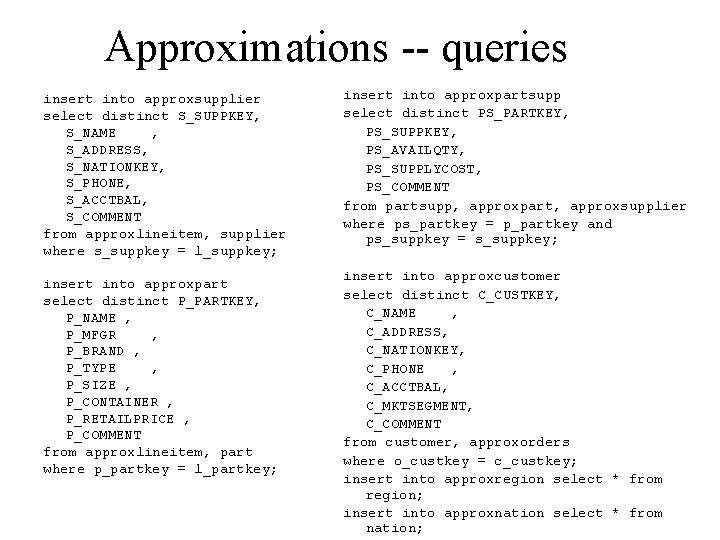
Approximations -- queries insert into approxsupplier select distinct S_SUPPKEY, S_NAME , S_ADDRESS, S_NATIONKEY, S_PHONE, S_ACCTBAL, S_COMMENT from approxlineitem, supplier where s_suppkey = l_suppkey; insert into approxpart select distinct P_PARTKEY, P_NAME , P_MFGR , P_BRAND , P_TYPE , P_SIZE , P_CONTAINER , P_RETAILPRICE , P_COMMENT from approxlineitem, part where p_partkey = l_partkey; insert into approxpartsupp select distinct PS_PARTKEY, PS_SUPPKEY, PS_AVAILQTY, PS_SUPPLYCOST, PS_COMMENT from partsupp, approxpart, approxsupplier where ps_partkey = p_partkey and ps_suppkey = s_suppkey; insert into approxcustomer select distinct C_CUSTKEY, C_NAME , C_ADDRESS, C_NATIONKEY, C_PHONE , C_ACCTBAL, C_MKTSEGMENT, C_COMMENT from customer, approxorders where o_custkey = c_custkey; insert into approxregion select * from region; insert into approxnation select * from nation;

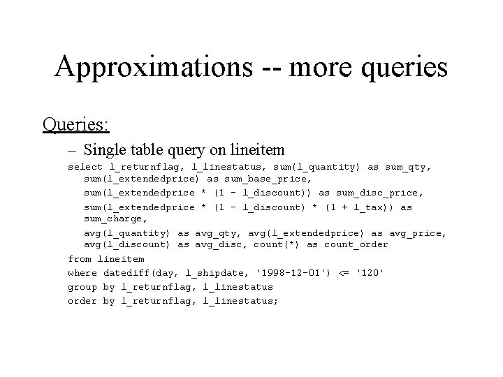
Approximations -- more queries Queries: – Single table query on lineitem select l_returnflag, l_linestatus, sum(l_quantity) as sum_qty, sum(l_extendedprice) as sum_base_price, sum(l_extendedprice * (1 - l_discount)) as sum_disc_price, sum(l_extendedprice * (1 - l_discount) * (1 + l_tax)) as sum_charge, avg(l_quantity) as avg_qty, avg(l_extendedprice) as avg_price, avg(l_discount) as avg_disc, count(*) as count_order from lineitem where datediff(day, l_shipdate, '1998 -12 -01') <= '120' group by l_returnflag, l_linestatus order by l_returnflag, l_linestatus;

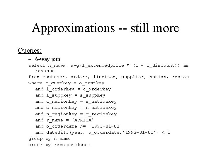
Approximations -- still more Queries: – 6 -way join select n_name, avg(l_extendedprice * (1 - l_discount)) as revenue from customer, orders, lineitem, supplier, nation, region where c_custkey = o_custkey and l_orderkey = o_orderkey and l_suppkey = s_suppkey and c_nationkey = s_nationkey and s_nationkey = n_nationkey and n_regionkey = r_regionkey and r_name = 'AFRICA' and o_orderdate >= '1993 -01 -01' and datediff(year, o_orderdate, '1993 -01 -01') < 1 group by n_name order by revenue desc;

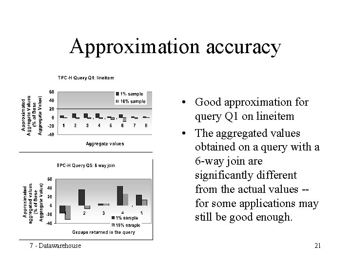
Approximation accuracy • Good approximation for query Q 1 on lineitem • The aggregated values obtained on a query with a 6 -way join are significantly different from the actual values -for some applications may still be good enough. 7 - Datawarehouse 21

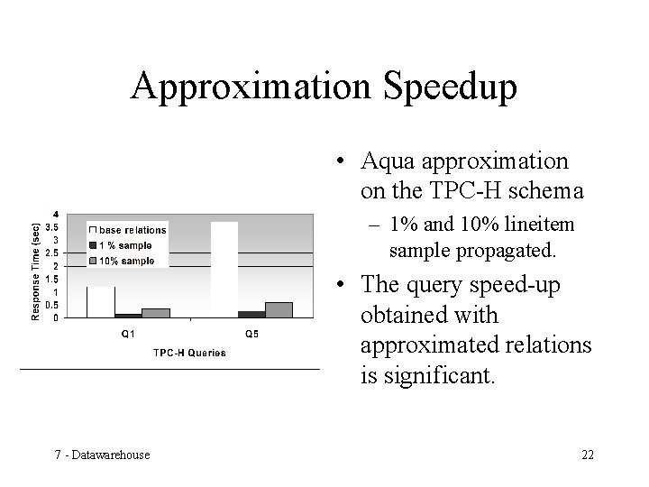
Approximation Speedup • Aqua approximation on the TPC-H schema – 1% and 10% lineitem sample propagated. • The query speed-up obtained with approximated relations is significant. 7 - Datawarehouse 22