Chapter 28 Real Options Land Value Land Value

Chapter 28 Real Options & Land Value

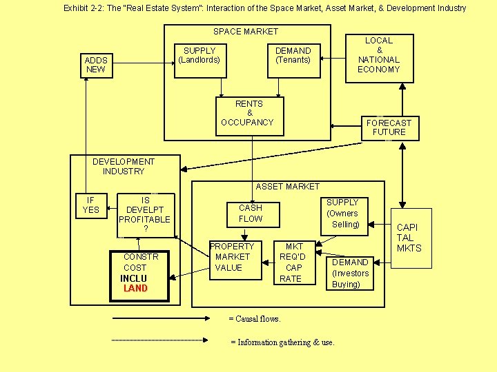
Land Value is perhaps the most fundamental topic in real estate: Recall the “Real Estate System” from Chapter 2. . .

Exhibit 2 -2: The “Real Estate System”: Interaction of the Space Market, Asset Market, & Development Industry SPACE MARKET SUPPLY (Landlords) ADDS NEW LOCAL & NATIONAL ECONOMY DEMAND (Tenants) RENTS & OCCUPANCY FORECAST FUTURE DEVELOPMENT INDUSTRY ASSET MARKET IF YES IS DEVELPT PROFITABLE ? CONSTR COST INCLU LAND SUPPLY (Owners Selling) CASH FLOW PROPERTY MARKET VALUE MKT REQ’D CAP RATE DEMAND (Investors Buying) = Causal flows. = Information gathering & use. CAPI TAL MKTS

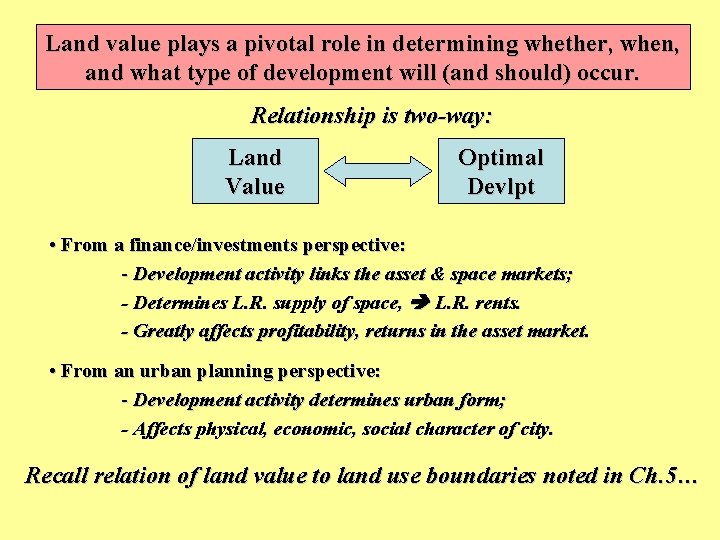
Land value plays a pivotal role in determining whether, when, and what type of development will (and should) occur. Relationship is two-way: Land Value Optimal Devlpt • From a finance/investments perspective: - Development activity links the asset & space markets; - Determines L. R. supply of space, L. R. rents. - Greatly affects profitability, returns in the asset market. • From an urban planning perspective: - Development activity determines urban form; - Affects physical, economic, social character of city. Recall relation of land value to land use boundaries noted in Ch. 5…

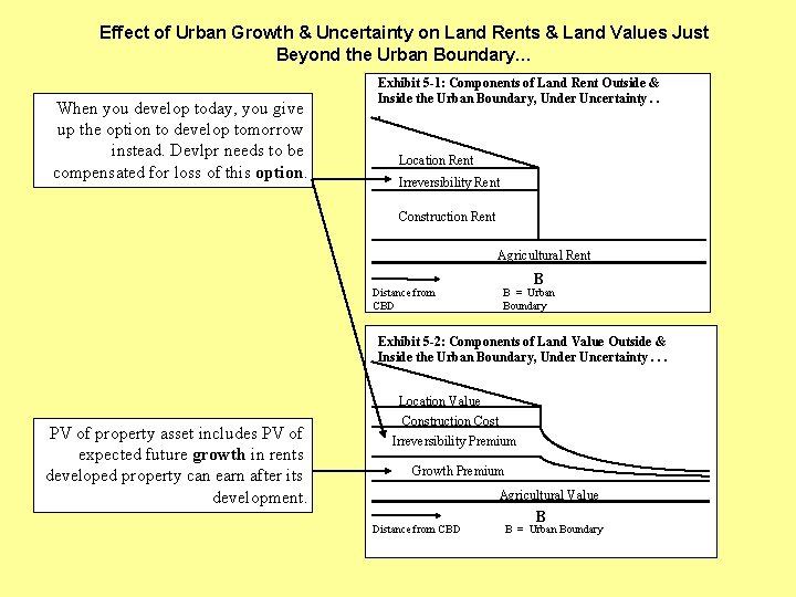
Effect of Urban Growth & Uncertainty on Land Rents & Land Values Just Beyond the Urban Boundary… When you develop today, you give up the option to develop tomorrow instead. Devlpr needs to be compensated for loss of this option. Exhibit 5 -1: Components of Land Rent Outside & Inside the Urban Boundary, Under Uncertainty. . . Location Rent Irreversibility Rent Construction Rent Agricultural Rent Distance from CBD B B = Urban Boundary Exhibit 5 -2: Components of Land Value Outside & Inside the Urban Boundary, Under Uncertainty. . . PV of property asset includes PV of expected future growth in rents developed property can earn after its development. Location Value Construction Cost Irreversibility Premium Growth Premium Agricultural Value Distance from CBD B B = Urban Boundary

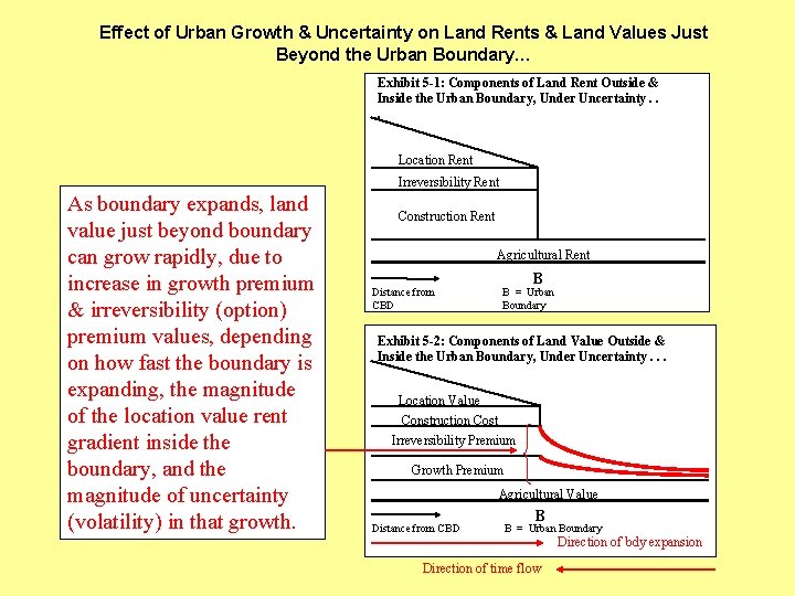
Effect of Urban Growth & Uncertainty on Land Rents & Land Values Just Beyond the Urban Boundary… Exhibit 5 -1: Components of Land Rent Outside & Inside the Urban Boundary, Under Uncertainty. . . Location Rent Irreversibility Rent As boundary expands, land value just beyond boundary can grow rapidly, due to increase in growth premium & irreversibility (option) premium values, depending on how fast the boundary is expanding, the magnitude of the location value rent gradient inside the boundary, and the magnitude of uncertainty (volatility) in that growth. Construction Rent Agricultural Rent Distance from CBD B B = Urban Boundary Exhibit 5 -2: Components of Land Value Outside & Inside the Urban Boundary, Under Uncertainty. . . Location Value Construction Cost Irreversibility Premium Growth Premium Agricultural Value Distance from CBD B B = Urban Boundary Direction of bdy expansion Direction of time flow

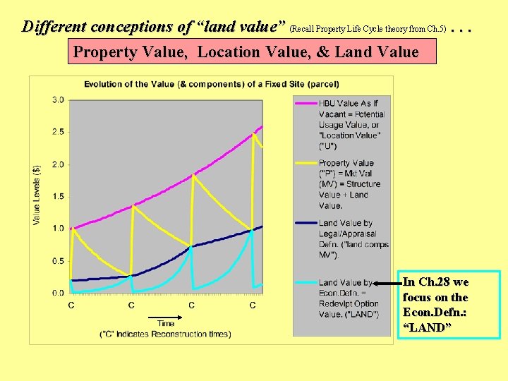
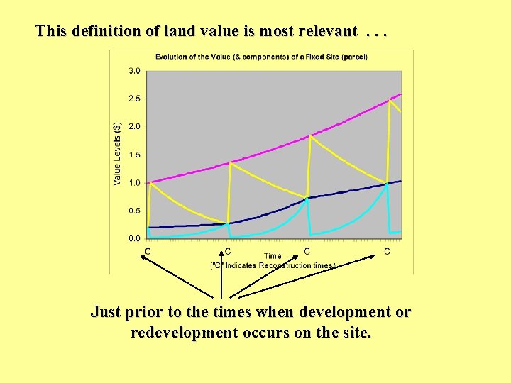
Different conceptions of “land value” (Recall Property Life Cycle theory from Ch. 5). . . Property Value, Location Value, & Land Value In Ch. 28 we focus on the Econ. Defn. : “LAND”

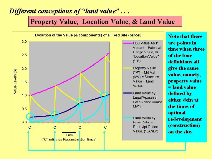
Different conceptions of “land value”. . . Property Value, Location Value, & Land Value Note that there are points in time when three of the four definitions all give the same value, namely, property value = land value defined by either defn at the times of optimal redevelopment (construction) on the site.

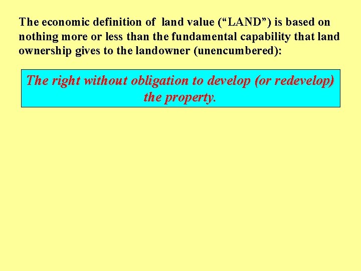
The economic definition of land value (“LAND”) is based on nothing more or less than the fundamental capability that land ownership gives to the landowner (unencumbered): The right without obligation to develop (or redevelop) the property.

This definition of land value is most relevant. . . Just prior to the times when development or redevelopment occurs on the site.

To understand the economic conception of land value, a famous theoretical development from financial economics is most useful: “Option Valuation Theory” (OVT) : In particular, a branch of that theory known a “Real Options”.

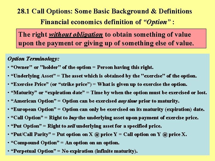
28. 1 Call Options: Some Basic Background & Definitions Financial economics definition of “Option” : The right without obligation to obtain something of value upon the payment or giving up of something else of value. Option Terminology: • “Owner" or "holder" of the option = Person having this right. • “Underlying Asset” = The asset which is obtained by the "exercise" of the option. • “Exercise Price” (or “strike price”) = What is given up to exercise the option. • “Maturity” or “expiration date” = Time by when the option must be exercised or lost. • “American Option” = Option can be exercised any time prior to maturity. • “European Option” = Option can only be exercised on its maturity (expiration) date. • “Call Option” = Right to buy the underlying asset upon payment of exercise price. • “Put Option” = Right to sell underlying asset for a specified price. • “Put/Call Parity” = Put option on X @ price Y = Call option on Y @ price X. • “Compound Option” = An option on an option. • “Perpetual Option” = No expiration (infinite maturity).

Option exercise is irreversible: Options can only be exercised once. Then the option is lost. OVT is a body of theory and methodology for quantitatively evaluating options. • For American options, this includes the problem of specifying the conditions when it is optimal to exercise the option: Optimal Exercise Policy. • For the land development option, this relates to the conditions when it is optimal to develop (or redevelop) the land.

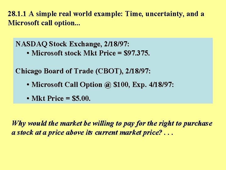
28. 1. 1 A simple real world example: Time, uncertainty, and a Microsoft call option. . . NASDAQ Stock Exchange, 2/18/97: • Microsoft stock Mkt Price = $97. 375. Chicago Board of Trade (CBOT), 2/18/97: • Microsoft Call Option @ $100, Exp. 4/18/97: • Mkt Price = $5. 00. Why would the market be willing to pay for the right to purchase a stock at a price above its current market price? . . .

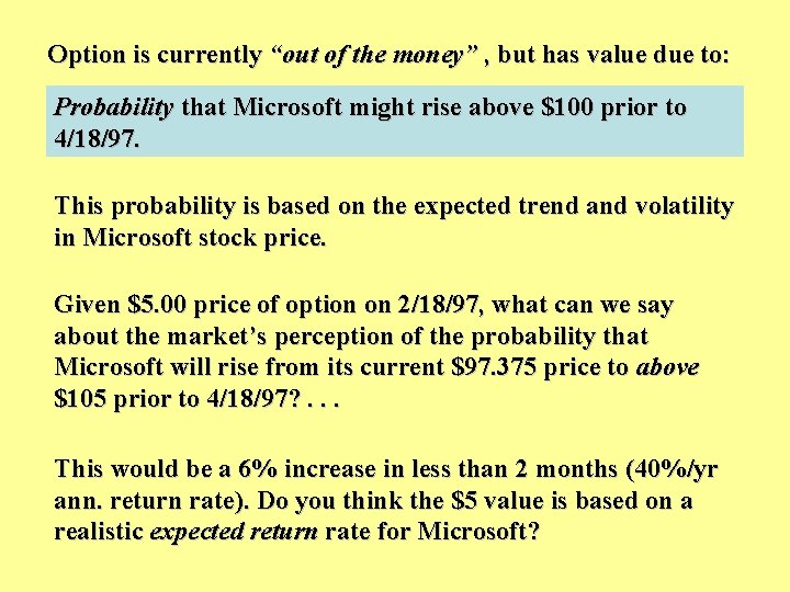
Option is currently “out of the money” , but has value due to: Probability that Microsoft might rise above $100 prior to 4/18/97. This probability is based on the expected trend and volatility in Microsoft stock price. Given $5. 00 price of option on 2/18/97, what can we say about the market’s perception of the probability that Microsoft will rise from its current $97. 375 price to above $105 prior to 4/18/97? . . . This would be a 6% increase in less than 2 months (40%/yr ann. return rate). Do you think the $5 value is based on a realistic expected return rate for Microsoft?

Options are “contingent claims” : • Have value only under certain “contingencies” (certain scenarios or outcomes or “states”), • Otherwise are worthless. • e. g. , If Microsoft rises above $100 prior to 4/18/97, then the call option (with the $100 strike price) will have value, otherwise it will expire worthless. Option values play upon two factors: Time Uncertainty

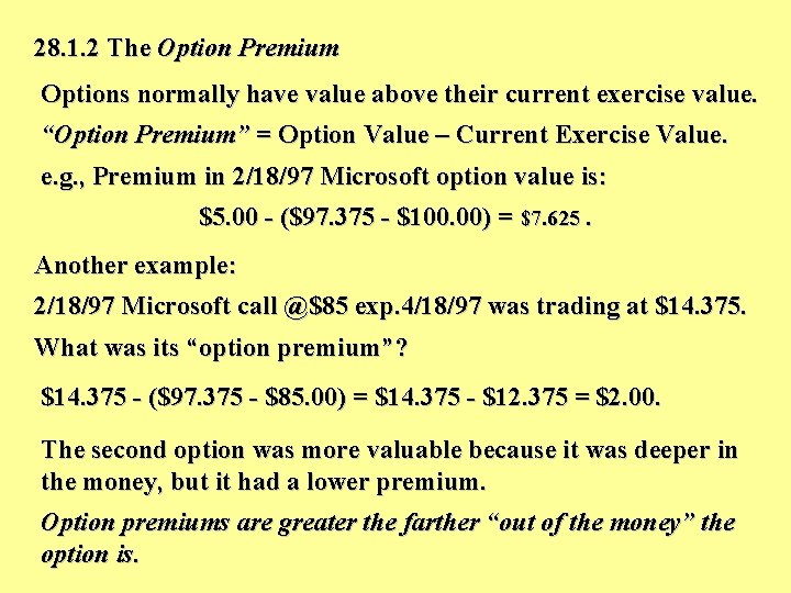
28. 1. 2 The Option Premium Options normally have value above their current exercise value. “Option Premium” = Option Value – Current Exercise Value. e. g. , Premium in 2/18/97 Microsoft option value is: $5. 00 - ($97. 375 - $100. 00) = $7. 625. Another example: 2/18/97 Microsoft call @$85 exp. 4/18/97 was trading at $14. 375. What was its “option premium”? $14. 375 - ($97. 375 - $85. 00) = $14. 375 - $12. 375 = $2. 00. The second option was more valuable because it was deeper in the money, but it had a lower premium. Option premiums are greater the farther “out of the money” the option is.

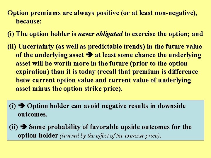
Option premiums are always positive (or at least non-negative), because: (i) The option holder is never obligated to exercise the option; and (ii) Uncertainty (as well as predictable trends) in the future value of the underlying asset at least some chance the underlying asset will be worth more in the future (prior to the option expiration) than it is today (recall that premium is difference betw current option value and current value of underlying asset minus the option strike price). (i) Option holder can avoid negative results in downside outcomes. (ii) Some probability of favorable upside outcomes for the option holder (levered by the effect of the exercise price).

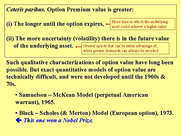
Ceteris paribus, Option Premium value is greater: (i) The longer until the option expires, More time in which the underlying asset could achieve a higher value (ii) The more uncertainty (volatility) there is in the future value Greater upside that can be taken advantage of, of the underlying asset. while greater downside can always be avoided. Such qualitative characterizations of option value have long been possible. But exact quantitative models of option value are technically difficult, and were not developed until the 1960 s & 70 s. • Samuelson – Mc. Kean Model (perpetual American warrant), 1965. • Black – Scholes (& Merton) Model (European option), 1973. This one won a Nobel Prize.

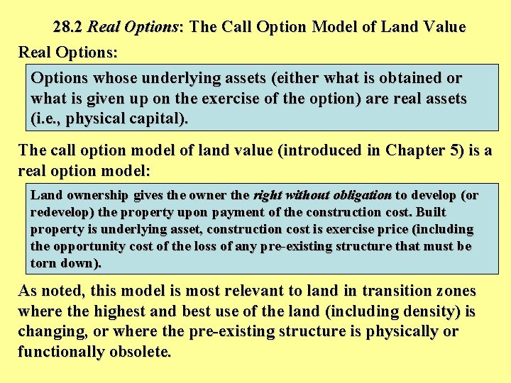
28. 2 Real Options: The Call Option Model of Land Value Real Options: Options whose underlying assets (either what is obtained or what is given up on the exercise of the option) are real assets (i. e. , physical capital). The call option model of land value (introduced in Chapter 5) is a real option model: Land ownership gives the owner the right without obligation to develop (or redevelop) the property upon payment of the construction cost. Built property is underlying asset, construction cost is exercise price (including the opportunity cost of the loss of any pre-existing structure that must be torn down). As noted, this model is most relevant to land in transition zones where the highest and best use of the land (including density) is changing, or where the pre-existing structure is physically or functionally obsolete.

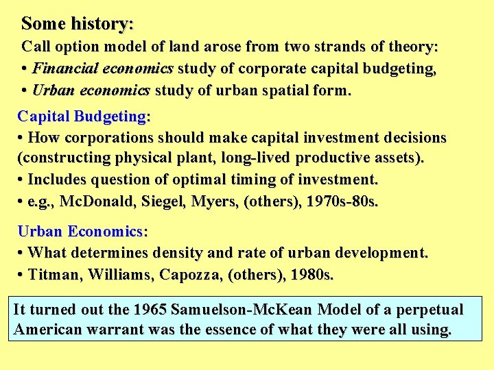
Some history: Call option model of land arose from two strands of theory: • Financial economics study of corporate capital budgeting, • Urban economics study of urban spatial form. Capital Budgeting: • How corporations should make capital investment decisions (constructing physical plant, long-lived productive assets). • Includes question of optimal timing of investment. • e. g. , Mc. Donald, Siegel, Myers, (others), 1970 s-80 s. Urban Economics: • What determines density and rate of urban development. • Titman, Williams, Capozza, (others), 1980 s. It turned out the 1965 Samuelson-Mc. Kean Model of a perpetual American warrant was the essence of what they were all using.

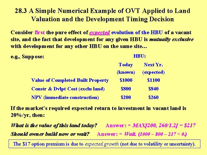
28. 3 A Simple Numerical Example of OVT Applied to Land Valuation and the Development Timing Decision Consider first the pure effect of expected evolution of the HBU of a vacant site, and the fact that development for any given HBU is mutually exclusive with development for any other HBU on the same site… HBU: e. g. , Suppose: Today (known) Next Yr. (expected) Value of Completed Built Property $1000 $1100 Constr & Dvlpt Cost (exclu land) $800 $840 NPV (immediate construction) $200 $260 If the market’s required expected return to investment in vacant land is 20%/yr, then: What is the value of this land today? Answer: = MAX[200, 260/1. 2] = $217 Should owner build now or wait? Answer: = Wait. (1000 – 800 – 217 < 0. ) The $17 option premium is due to expected growth (not due to volatility or uncertainty).

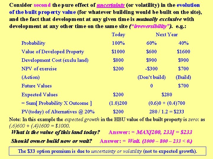
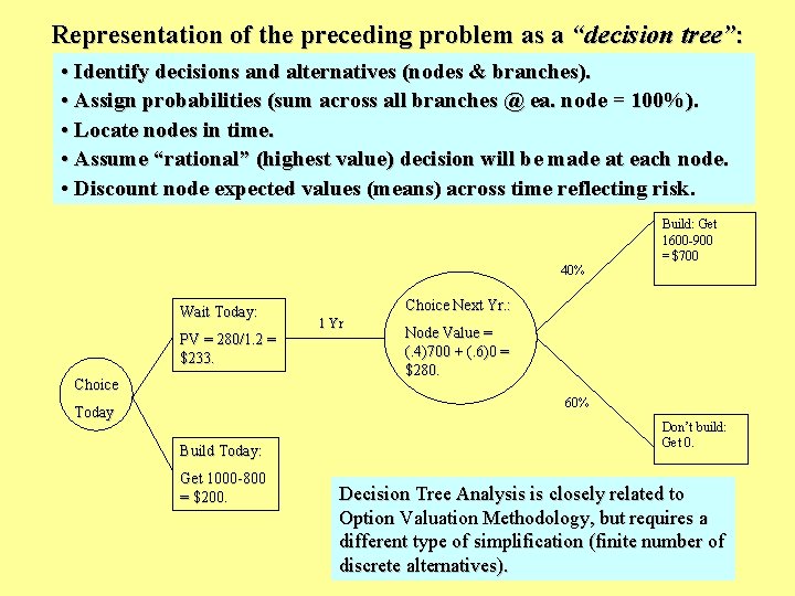
Consider second the pure effect of uncertainty (or volatility) in the evolution of the built property value (for whatever building would be built on the site), and the fact that development at any given time is mutually exclusive with development at any other time on the same site (“irreversibility”). e. g. : Today Next Year Probability 100% 60% 40% Value of Developed Property $1000 $600 $1600 Development Cost (exclu land) $800 $900 NPV of exercise $200 -$300 $700 (Don’t build) (Build) 0 $700 (Action) Future Values Expected Values = Sum[ Probability X Outcome ] $200 $280 (1. 0)200 (0. 6)0 + (0. 4)700 PV(today) of Alternatives @ 20% $200 280 / 1. 2 = $233 Note: In this example the expected growth in the HBU value of the built property is zero: as (. 6)600 + (. 4)1600 = $1000. What is the value of this land today? Answer: = MAX[200, 233] = $233 Should owner build now or wait? Answer: = Wait. (1000 – 800 – 233 < 0. ) The $33 option premium is due to uncertainty or volatility (not to expected growth).

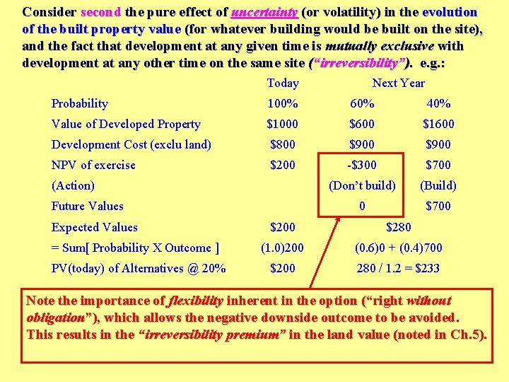
Consider second the pure effect of uncertainty (or volatility) in the evolution of the built property value (for whatever building would be built on the site), and the fact that development at any given time is mutually exclusive with development at any other time on the same site (“irreversibility”). e. g. : Today Next Year Probability 100% 60% 40% Value of Developed Property $1000 $600 $1600 Development Cost (exclu land) $800 $900 NPV of exercise $200 -$300 $700 (Don’t build) (Build) 0 $700 (Action) Future Values Expected Values $200 $280 = Sum[ Probability X Outcome ] (1. 0)200 (0. 6)0 + (0. 4)700 PV(today) of Alternatives @ 20% $200 280 / 1. 2 = $233 Note the importance of flexibility inherent in the option (“right without obligation”), which allows the negative downside outcome to be avoided. This results in the “irreversibility premium” in the land value (noted in Ch. 5).

Representation of the preceding problem as a “decision tree”: • Identify decisions and alternatives (nodes & branches). • Assign probabilities (sum across all branches @ ea. node = 100%). • Locate nodes in time. • Assume “rational” (highest value) decision will be made at each node. • Discount node expected values (means) across time reflecting risk. 40% Wait Today: PV = 280/1. 2 = $233. Choice Build: Get 1600 -900 = $700 Choice Next Yr. : 1 Yr Node Value = (. 4)700 + (. 6)0 = $280. 60% Today Build Today: Get 1000 -800 = $200. Don’t build: Get 0. Decision Tree Analysis is closely related to Option Valuation Methodology, but requires a different type of simplification (finite number of discrete alternatives).

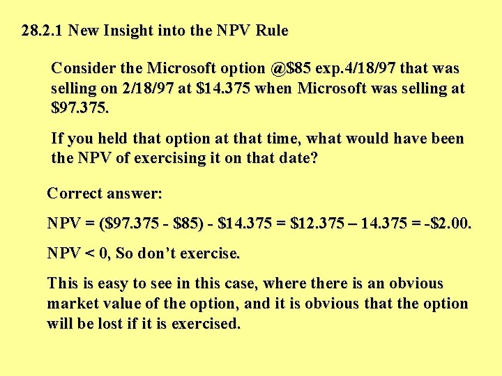
28. 2. 1 New Insight into the NPV Rule Consider the Microsoft option @$85 exp. 4/18/97 that was selling on 2/18/97 at $14. 375 when Microsoft was selling at $97. 375. If you held that option at that time, what would have been the NPV of exercising it on that date? Correct answer: NPV = ($97. 375 - $85) - $14. 375 = $12. 375 – 14. 375 = -$2. 00. NPV < 0, So don’t exercise. This is easy to see in this case, where there is an obvious market value of the option, and it is obvious that the option will be lost if it is exercised.

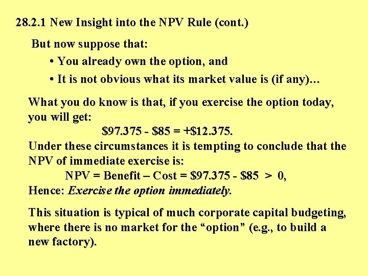
28. 2. 1 New Insight into the NPV Rule (cont. ) But now suppose that: • You already own the option, and • It is not obvious what its market value is (if any)… What you do know is that, if you exercise the option today, you will get: $97. 375 - $85 = +$12. 375. Under these circumstances it is tempting to conclude that the NPV of immediate exercise is: NPV = Benefit – Cost = $97. 375 - $85 > 0, Hence: Exercise the option immediately. This situation is typical of much corporate capital budgeting, where there is no market for the “option” (e. g. , to build a new factory).

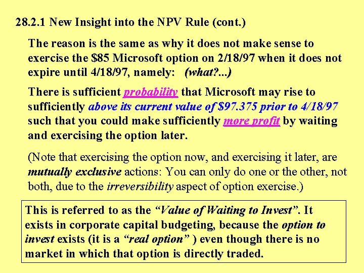
28. 2. 1 New Insight into the NPV Rule (cont. ) But the fact that there is no market for the option does not mean that the option does not exist, or that it does not have investment value (IV), or that it will not be lost upon exercise (remember irreversibility). Indeed, the optimal investment decision is (in the abovedescribed circumstances) to wait before investing (in the new factory or whatever), even though the NPV of immediate exercise appears to be positive. Why?

28. 2. 1 New Insight into the NPV Rule (cont. ) The reason is the same as why it does not make sense to exercise the $85 Microsoft option on 2/18/97 when it does not expire until 4/18/97, namely: (what? . . . ) There is sufficient probability that Microsoft may rise to sufficiently above its current value of $97. 375 prior to 4/18/97 such that you could make sufficiently more profit by waiting and exercising the option later. (Note that exercising the option now, and exercising it later, are mutually exclusive actions: You can only do one or the other, not both, due to the irreversibility aspect of option exercise. ) This is referred to as the “Value of Waiting to Invest”. It exists in corporate capital budgeting, because the option to invest exists (it is a “real option” ) even though there is no market in which that option is directly traded.

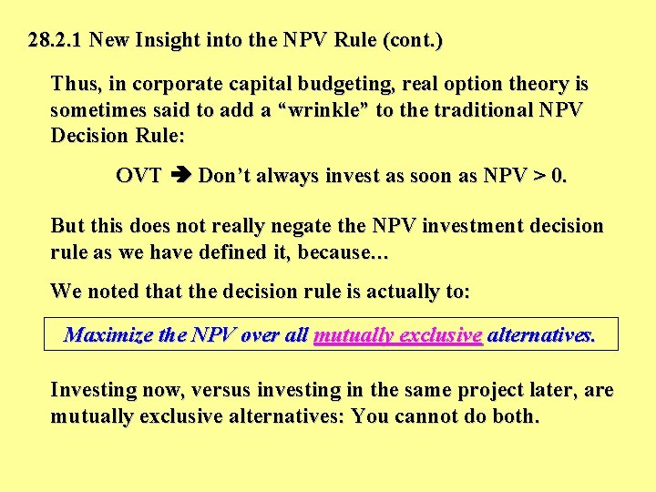
28. 2. 1 New Insight into the NPV Rule (cont. ) Thus, in corporate capital budgeting, real option theory is sometimes said to add a “wrinkle” to the traditional NPV Decision Rule: OVT Don’t always invest as soon as NPV > 0. But this does not really negate the NPV investment decision rule as we have defined it, because… We noted that the decision rule is actually to: Maximize the NPV over all mutually exclusive alternatives. Investing now, versus investing in the same project later, are mutually exclusive alternatives: You cannot do both.

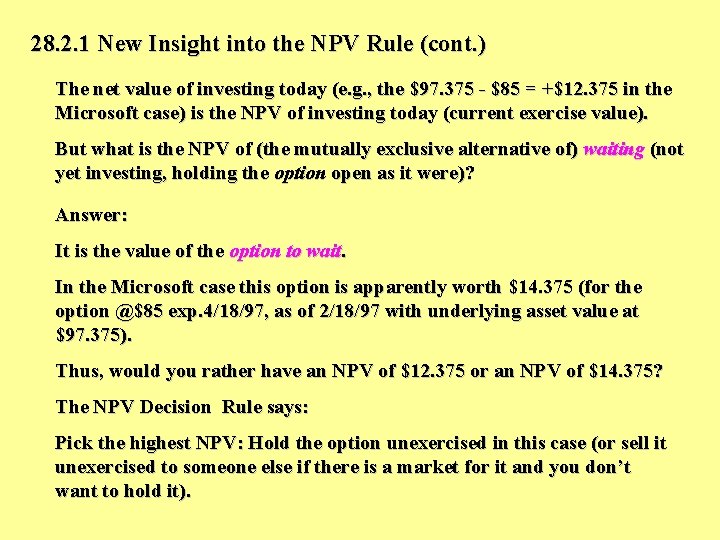
28. 2. 1 New Insight into the NPV Rule (cont. ) The net value of investing today (e. g. , the $97. 375 - $85 = +$12. 375 in the Microsoft case) is the NPV of investing today (current exercise value). But what is the NPV of (the mutually exclusive alternative of) waiting (not yet investing, holding the option open as it were)? Answer: It is the value of the option to wait. In the Microsoft case this option is apparently worth $14. 375 (for the option @$85 exp. 4/18/97, as of 2/18/97 with underlying asset value at $97. 375). Thus, would you rather have an NPV of $12. 375 or an NPV of $14. 375? The NPV Decision Rule says: Pick the highest NPV: Hold the option unexercised in this case (or sell it unexercised to someone else if there is a market for it and you don’t want to hold it).

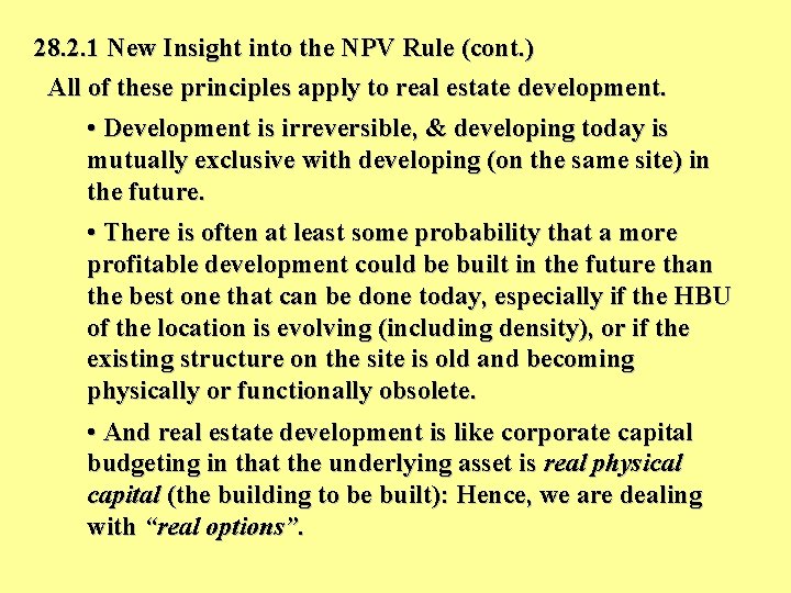
28. 2. 1 New Insight into the NPV Rule (cont. ) All of these principles apply to real estate development. • Development is irreversible, & developing today is mutually exclusive with developing (on the same site) in the future. • There is often at least some probability that a more profitable development could be built in the future than the best one that can be done today, especially if the HBU of the location is evolving (including density), or if the existing structure on the site is old and becoming physically or functionally obsolete. • And real estate development is like corporate capital budgeting in that the underlying asset is real physical capital (the building to be built): Hence, we are dealing with “real options”.

28. 2. 1 New Insight into the NPV Rule (cont. ) However, there is an important difference between the real estate development case and the corporate capital budgeting case… Unlike the corporate capital budgeting case (but more like the case of the Microsoft option traded on the CBOT), in real estate development there is a functioning market for the real option, namely: (What? . . . ) THE LAND MARKET If the land market is functioning well, the market value of land should reflect the option value inherent in the land ownership, including the value of any “option premium” (the component above the current exercise value of the option).

28. 2. 1 New Insight into the NPV Rule (cont. ) In computing the NPV of any potential development project, the current opportunity cost of the land must be included as one of the costs of the project. That is, the current market value of the land should be counted on the cost side of the NPV equation, what the land could be sold for today (which may differ from its historical cost). Thus, when applied properly, the NPV rule still holds, and is relevant for evaluating real estate development projects. CAVEAT: Although a well functioning land market normally exists, in some cases it doesn’t, and it is never as perfect and efficient as the CBOT Options Exchange in which the Microsoft options that we considered were traded.

Footnote: There may be special circumstances in which the developer’s opportunity cost does not exactly reflect the current market value of the land unencumbered. e. g. , Developer does not own the land outright, has only a finite-lived “use-it-or-lose-it” option to develop on the land. This option would be less valuable than unencumbered ownership of the land that would allow development at any time (more flexibility to wait to invest). But the market value of the land thusly encumbered (by the option granted to the developer) would also be less than the value of the unencumbered land. The two values combined might be less than the unencumbered value of the land, because of the loss in flexibility in the timing of optimal construction (due to the division of the unencumbered ownership rights). The “social value” of the land might be defined as the unencumbered market value.

The value of newly-built property will include the (remaining) economic value of the land (“LAND”), but: • This land value will now be minus its initial development option value (which has been exercised), • It will include the redevelopment (or abandonment) option value. • However, this redevelopment option value will normally be quite small in a newly developed property (recall property “life -cycle” chart). Speaking in terms of the economic definition of land value, based on its option value.

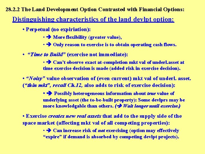
28. 2. 2 The Land Development Option Contrasted with Financial Options: Distinguishing characteristics of the land devlpt option: • Perpetual (no expiriation): • More flexibility (greater value), • Only reason to exercise is to obtain operating cash flows. • “Time to Build” (exercise not immediate): • Can’t observe exact at-completion mkt val of underl. asset at time exercise decision is made (added risk in exercise decision). • “Noisy” value observation of (even current) mkt val of underl. asset. (“thin mkt”, recall Ch. 12, also adds to risk of exercise decision): • Possibly heterogeneous information about true value of underlying asset (the to-be-built property): Some devlprs may be more knowledgable than others. ( Wait longer until exercise. ) • Exercise creates new real assets that add to the supply side of the space market (affecting mkt val of all competing properties): • Can increase risk of not exercising (option may effectively “expire” if demand is absorbed by competing devlpt projects).

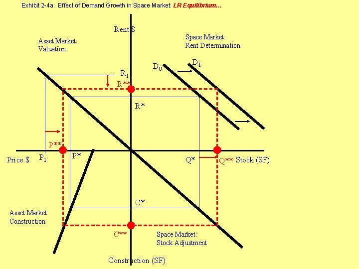
What the real option theory of land development can tell us about the “overbuilding phenomenon”. . . What is the “overbuilding phenomenon”? . . . The widely observed tendency for commercial real estate markets to periodically become “overbuilt”, that is, characterized by excess supply (abnormally high vacancy, downward pressure on rents), due to excessive speculative development of new buildings. Recall that in Chapter 2 we discussed an explanation for this “cyclicality” phenomenon using the “ 4 -Quadrant Diagram”, based on the existence of myopic behavior (not just lack of perfect foresight, but some degree of irrational expectations) on the part of investors and developers in the system. . .

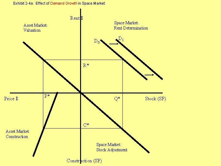
Exhibit 2 -4 a: Effect of Demand Growth in Space Market: Rent $ Space Market: Rent Determination Asset Market: Valuation D 0 D 1 R* Price $ P* Q* C* Asset Market: Construction Space Market: Stock Adjustment Construction (SF) Stock (SF)

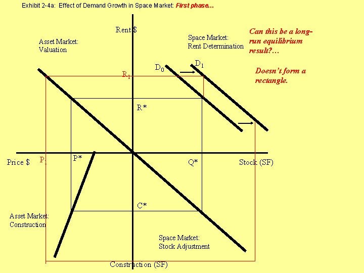
Exhibit 2 -4 a: Effect of Demand Growth in Space Market: First phase… Rent $ Can this be a long- Space Market: run equilibrium Rent Determination Asset Market: Valuation result? … D 0 R 1 Doesn’t form a rectangle. R* Price $ P 1 P* Q* C* Asset Market: Construction Space Market: Stock Adjustment Construction (SF) Stock (SF)

Exhibit 2 -4 a: Effect of Demand Growth in Space Market: LR Equilibrium… Rent $ Space Market: Rent Determination Asset Market: Valuation D 0 R 1 R** D 1 R* P** Price $ P 1 P* Q* C* Asset Market: Construction C** Space Market: Stock Adjustment Construction (SF) Q** Stock (SF)

Real option theory offers several explanations for why/how overbuilding can be due to completely rational (i. e. , profitmaximizing) behavior on the part of developers (landowners): 1. “Cascades”: Noisy observations of the mkt values of the underlying assets (comparable built properties), combined with heterogeneous developer knowledge about the “true” value, causes a follow-the-leader type effect, in which developers wait longer than they otherwise would to develop, and then they all rush in as soon as the first (presumably most knowledgeable) developer reveals his knowledge by commencing development. 2. “Lumpy supply & first out of the gate”: Economies of scale in building size, combined with finite user demand the fact that option exercise creates real physical capital, leads to early exercise of the development option to preclude loss (expiration) of the option if a competitor builds first. 3. “Long-term leasing option”: The cost of having empty space in a new building may be less than it first appears in space markets characterized by long-term leases, as it gives the landlord a leasing option, that has value prior to its “exercise” (in the signing of a lease contract): Volatility in the rental mkt may bring better long-term lease deals in the future.

28. 4 The Samuelson-Mc. Kean Formula Applied to Land Value as a Development Option Compared to Decision Tree Analysis, Option Valuation Theory (OVT) can provide a more complete formulation of the value and optimal exercise strategy for contingent claims such as land ownership. But OVT also requires simplifying assumptions: • Frictionless markets; • “Random Walk” market value of underlying asset; • Normally distributed returns to underlying asset; • Known parameter values (e. g. , volatility of underlying asset). The simplest option valuation formula is also the first one developed, and the one that is most relevant to land valuation: The Samuelson-Mc. Kean Formula Developed by Nobel Prize winning economist Paul Samuelson and his mathematician partner Henry Mc. Kean, at MIT in 1965, as a model of a “perpetual American warrant”.

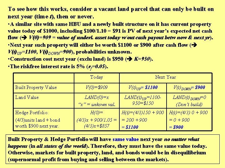
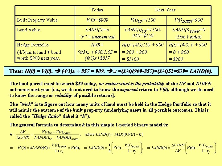
To see how this works, consider a vacant land parcel that can only be built on next year (time t), then or never. • A similar site with same HBU and a newly built structure on it has current property value today of $1000, including $100/1. 10 = $91 is PV of next year’s expected net cash flow ( V(0)=909 = value of underl. asset today w/out cash payout betw now & next yr). • Next year such property will either be worth $1100 or $900 after cash flow ( V(t)UP=1100, V(t)DOWN=900), probabilities unknown. • Construction cost next year (exclu land) is $950 ( K=950). • The riskfree interest rate is 5% (rf=0. 05). Today Built Property Value Next Year V(0)=$909 V(t)UP= $1100 V(t)DOWN= $900 Land Value LAND(0)=x “x” = unkown val. LAND(t)UP=1100950=$150 LAND(t)DOWN=0 (Don’t build) Hedge Portfolio: (4/3)units land + bond worth $900 next year. H(0)= H(t)=(4/3)150 + 900 (4/3)x + 900/1. 05 = = 200 + 900 (4/3)x+$857 = $1100 H(t)=(4/3) 0 + 900 = $900 Built Property & Hedge Portfolio will have same value next year no matter what happens (in all states of the world). Therefore, they must have the same value today. Otherwise, markets for built property, land, and bonds would be in disequilibrium (supernormal profit from buying and selling between the markets).

Today Built Property Value Next Year V(0)=$909 V(t)UP=1100 V(t)DOWN=900 Land Value LAND(0)=x “x” = unkown val. LAND(t)UP=1100950=$150 LAND(t)DOWN=0 (Don’t build) Hedge Portfolio: (4/3)units land + bond worth $900 next year. H(0)= H(t)=(4/3)150 + 900 (4/3)x + 900/1. 05 = = 200 + 900 (4/3)x+$857 = $1100 H(t)=(4/3) 0 + 900 = $900 Thus: H(0) = V(0). (4/3)x + 857 = 909. x =(3/4)(909 -857)=(3/4)52=$39= LAND(0). The land parcel must be worth $39 today, no matter what is the probability of the UP and DOWN outcomes next year [i. e. , we do not need to know the expected return to V(0), although we do need to know the range or volatility of possible returns]. The “trick” is to figure out how many units of land must be held in the Hedge Portfolio so that it will mimic the outcome of the built property (underlying asset) in all possible outcomes. This is called the “Hedge Ratio” (label it “h”). The general formula to determine h in this simple 1 -period binary model is:

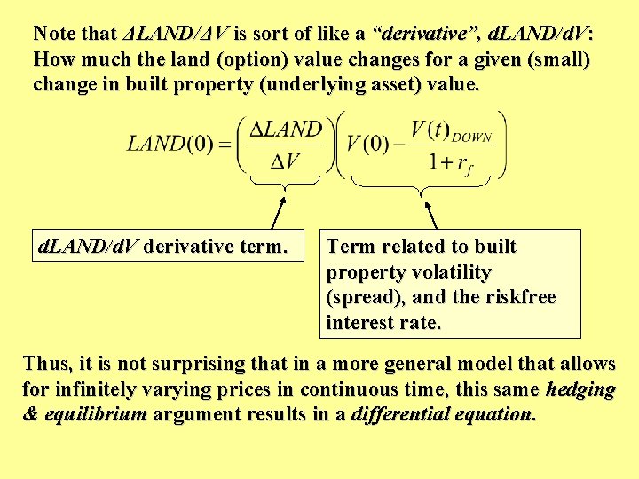
Note that ΔLAND/ΔV is sort of like a “derivative”, d. LAND/d. V: How much the land (option) value changes for a given (small) change in built property (underlying asset) value. d. LAND/d. V derivative term. Term related to built property volatility (spread), and the riskfree interest rate. Thus, it is not surprising that in a more general model that allows for infinitely varying prices in continuous time, this same hedging & equilibrium argument results in a differential equation.

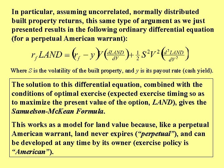
In particular, assuming uncorrelated, normally distributed built property returns, this same type of argument as we just presented results in the following ordinary differential equation (for a perpetual American warrant): Where S is the volatility of the built property, and y is its payout rate (cash yield). The solution to this differential equation, combined with the conditions of optimal exercise (expected exercise timing so as to maximize the present value of the option, LAND), gives the Samuelson-Mc. Kean Formula. This works as a model for land value because, like a perpetual American warrant, land never expires (“perpetual”), and can be developed at any time by its owner (exercise policy is “American”).

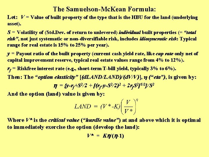
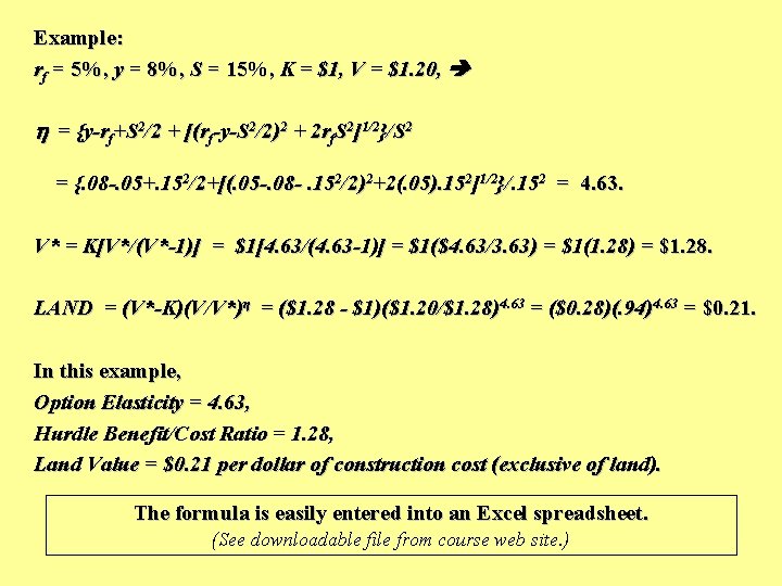
The Samuelson-Mc. Kean Formula: Let: V = Value of built property of the type that is the HBU for the land (underlying asset). S = Volatility of (Std. Dev. of return to unlevered) individual built properties (= “total risk”, not just systematic or non-diversifiable risk, includes idiosyncratic risk: Typical range for real estate is 15% to 25% per year). y = Payout ratio of the built property (current cash yield rate, like cap rate only net of capital improvement reserve, typical real estate values range from 4% to 12%). rf = Riskfree interest rate (e. g. , short-term T-bill yield, typically 3% to 6%). Then: The “option elasticity” [(d. LAND/LAND)/(d. V/V)], η (“eta”), is given by: = {y-rf+S 2/2 + [(rf-y-S 2/2)2 + 2 rf. S 2]1/2}/S 2 And the option (land) value is given by: Where V* is the critical value (“hurdle value”) at and above which it is optimal to immediately exercise the option (develop the land): V* = K /( -1)

Example: rf = 5%, y = 8%, S = 15%, K = $1, V = $1. 20, = {y-rf+S 2/2 + [(rf-y-S 2/2)2 + 2 rf. S 2]1/2}/S 2 = {. 08 -. 05+. 152/2+[(. 05 -. 08 -. 152/2)2+2(. 05). 152]1/2}/. 152 = 4. 63. V* = K[V*/(V*-1)] = $1[4. 63/(4. 63 -1)] = $1($4. 63/3. 63) = $1(1. 28) = $1. 28. LAND = (V*-K)(V/V*)η = ($1. 28 - $1)($1. 20/$1. 28)4. 63 = ($0. 28)(. 94)4. 63 = $0. 21. In this example, Option Elasticity = 4. 63, Hurdle Benefit/Cost Ratio = 1. 28, Land Value = $0. 21 per dollar of construction cost (exclusive of land). The formula is easily entered into an Excel spreadsheet. (See downloadable file from course web site. )

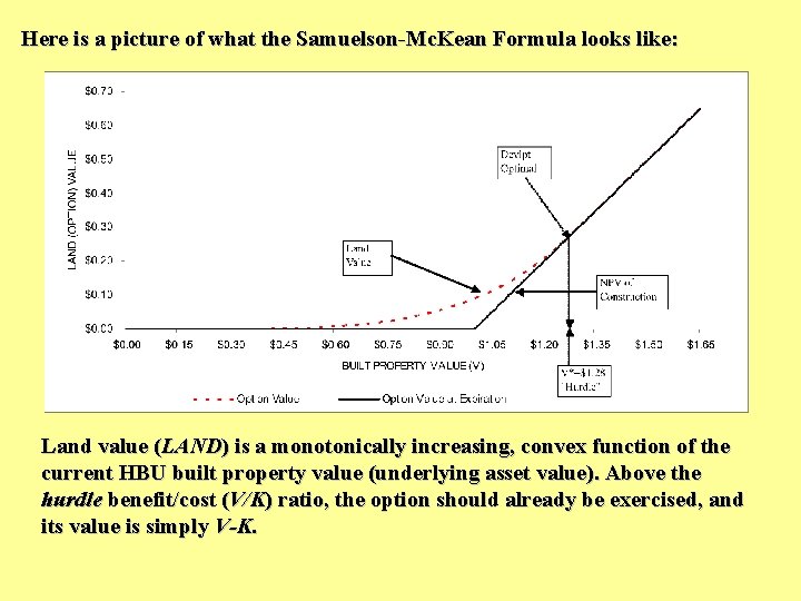
Here is a picture of what the Samuelson-Mc. Kean Formula looks like: Land value (LAND) is a monotonically increasing, convex function of the current HBU built property value (underlying asset value). Above the hurdle benefit/cost (V/K) ratio, the option should already be exercised, and its value is simply V-K.

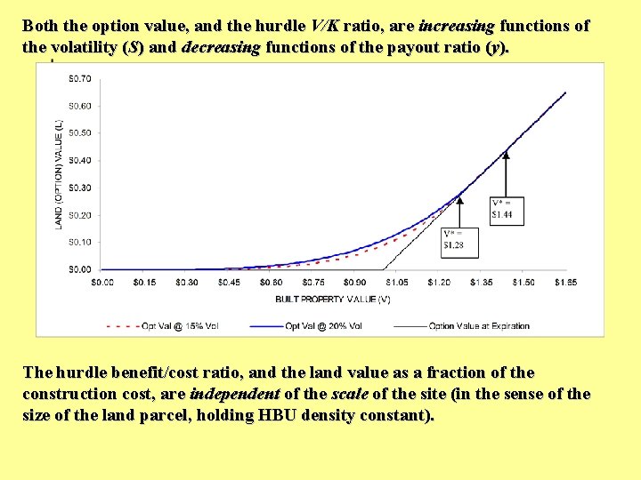
Both the option value, and the hurdle V/K ratio, are increasing functions of the volatility (S) and decreasing functions of the payout ratio (y). The hurdle benefit/cost ratio, and the land value as a fraction of the construction cost, are independent of the scale of the site (in the sense of the size of the land parcel, holding HBU density constant).

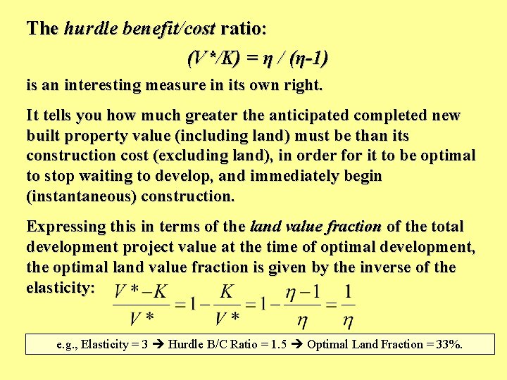
The hurdle benefit/cost ratio: (V*/K) = η / (η-1) is an interesting measure in its own right. It tells you how much greater the anticipated completed new built property value (including land) must be than its construction cost (excluding land), in order for it to be optimal to stop waiting to develop, and immediately begin (instantaneous) construction. Expressing this in terms of the land value fraction of the total development project value at the time of optimal development, the optimal land value fraction is given by the inverse of the elasticity: e. g. , Elasticity = 3 Hurdle B/C Ratio = 1. 5 Optimal Land Fraction = 33%.

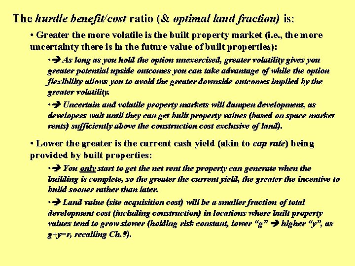
The hurdle benefit/cost ratio (& optimal land fraction) is: • Greater the more volatile is the built property market (i. e. , the more uncertainty there is in the future value of built properties): • As long as you hold the option unexercised, greater volatility gives you greater potential upside outcomes you can take advantage of while the option flexibility allows you to avoid the greater downside outcomes implied by the greater volatility. • Uncertain and volatile property markets will dampen development, as developers wait until they can get built property values (based on space market rents) sufficiently above the construction cost exclusive of land). • Lower the greater is the current cash yield (akin to cap rate) being provided by built properties: • You only start to get the net rent the property can generate when the building is complete, so the greater the current yield, the greater the incentive to build sooner rather than later. • Land value (site acquisition cost) will be a smaller fraction of total development cost (including construction) in locations where built property values tend to grow slower (holding risk constant, lower “g” higher “y”, as g+y=r, recalling Ch. 9).

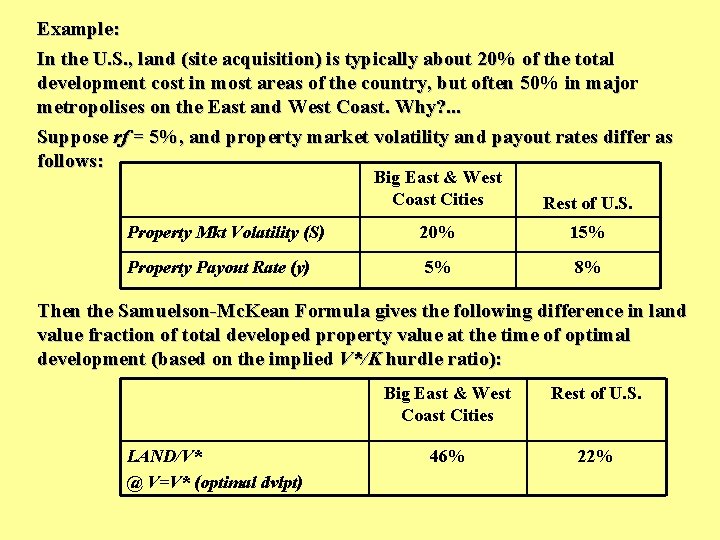
Example: In the U. S. , land (site acquisition) is typically about 20% of the total development cost in most areas of the country, but often 50% in major metropolises on the East and West Coast. Why? . . . Suppose rf = 5%, and property market volatility and payout rates differ as follows: Big East & West Coast Cities Rest of U. S. Property Mkt Volatility (S) 20% 15% Property Payout Rate (y) 5% 8% Then the Samuelson-Mc. Kean Formula gives the following difference in land value fraction of total developed property value at the time of optimal development (based on the implied V*/K hurdle ratio): LAND/V* @ V=V* (optimal dvlpt) Big East & West Coast Cities Rest of U. S. 46% 22%

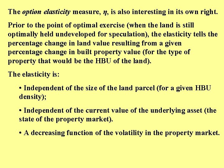
The option elasticity measure, η, is also interesting in its own right. Prior to the point of optimal exercise (when the land is still optimally held undeveloped for speculation), the elasticity tells the percentage change in land value resulting from a given percentage change in built property value (for the type of property that would be the HBU of the land). The elasticity is: • Independent of the size of the land parcel (for a given HBU density); • Independent of the current value of the underlying asset (the state of the property market). • A decreasing function of the volatility in the property market.

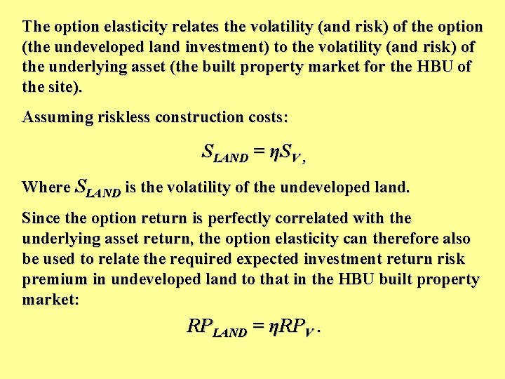
The option elasticity relates the volatility (and risk) of the option (the undeveloped land investment) to the volatility (and risk) of the underlying asset (the built property market for the HBU of the site). Assuming riskless construction costs: SLAND = ηSV , Where SLAND is the volatility of the undeveloped land. Since the option return is perfectly correlated with the underlying asset return, the option elasticity can therefore also be used to relate the required expected investment return risk premium in undeveloped land to that in the HBU built property market: RPLAND = ηRPV.

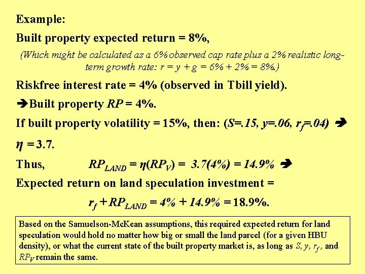
Example: Built property expected return = 8%, (Which might be calculated as a 6% observed cap rate plus a 2% realistic longterm growth rate: r = y + g = 6% + 2% = 8%. ) Riskfree interest rate = 4% (observed in Tbill yield). Built property RP = 4%. If built property volatility = 15%, then: (S=. 15, y=. 06, rf=. 04) η = 3. 7. Thus, RPLAND = η(RPV) = 3. 7(4%) = 14. 9% Expected return on land speculation investment = rf + RPLAND = 4% + 14. 9% = 18. 9%. Based on the Samuelson-Mc. Kean assumptions, this required expected return for land speculation would hold no matter how big or small the land parcel (for a given HBU density), or what the current state of the built property market is, as long as S, y, rf , and RPV remain the same.

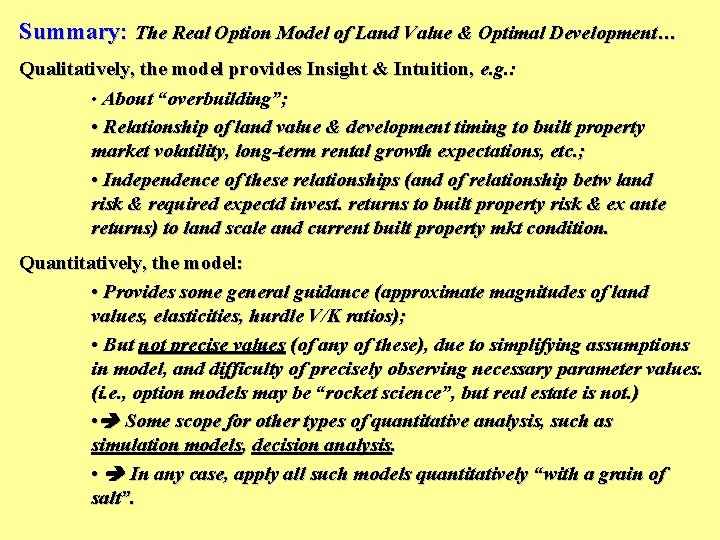
Summary: The Real Option Model of Land Value & Optimal Development… Qualitatively, the model provides Insight & Intuition, e. g. : • About “overbuilding”; • Relationship of land value & development timing to built property market volatility, long-term rental growth expectations, etc. ; • Independence of these relationships (and of relationship betw land risk & required expectd invest. returns to built property risk & ex ante returns) to land scale and current built property mkt condition. Quantitatively, the model: • Provides some general guidance (approximate magnitudes of land values, elasticities, hurdle V/K ratios); • But not precise values (of any of these), due to simplifying assumptions in model, and difficulty of precisely observing necessary parameter values. (i. e. , option models may be “rocket science”, but real estate is not. ) • Some scope for other types of quantitative analysis, such as simulation models, decision analysis. • In any case, apply all such models quantitatively “with a grain of salt”.