From financial options to real options 3 Real

From financial options to real options 3. Real option valuations Prof. André Farber Solvay Business School ESCP March 10, 2000 Valuing real options 1

Back to Portlandia Ale • Portlandia Ale had 2 different options: – the option to launch (a 2 -year European call option) • value can be calculated with BS – the option to abandon (a 2 -year American option) • How to value this American option? – No closed form solution – Numerical method: use recursive model based on binomial evolution of value – At each node, check whether to exercice or not. – Option value = Max(Option exercised, option alive) Valuing real options 2

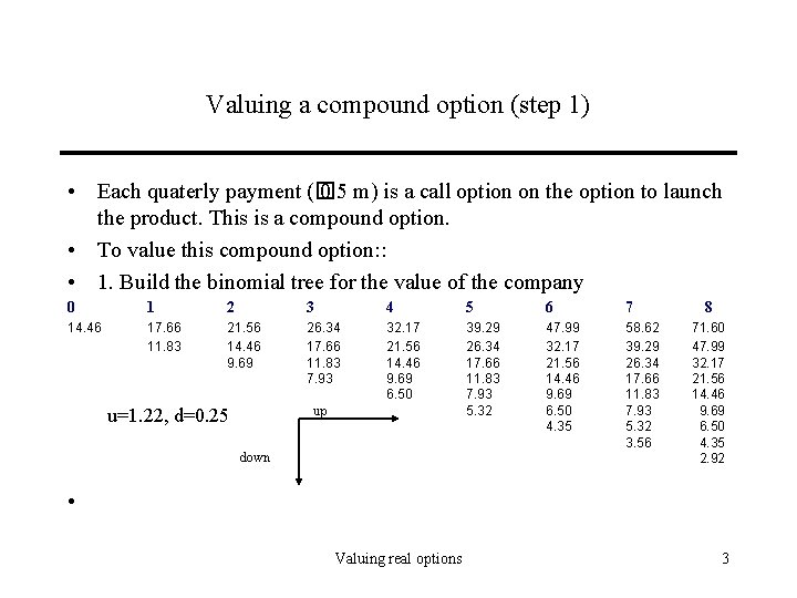
Valuing a compound option (step 1) • Each quaterly payment (� 0. 5 m) is a call option on the option to launch the product. This is a compound option. • To value this compound option: : • 1. Build the binomial tree for the value of the company 0 1 2 3 4 5 6 7 14. 46 17. 66 11. 83 21. 56 14. 46 9. 69 26. 34 17. 66 11. 83 7. 93 32. 17 21. 56 14. 46 9. 69 6. 50 39. 29 26. 34 17. 66 11. 83 7. 93 5. 32 47. 99 32. 17 21. 56 14. 46 9. 69 6. 50 4. 35 58. 62 39. 29 26. 34 17. 66 11. 83 7. 93 5. 32 3. 56 up u=1. 22, d=0. 25 down 8 71. 60 47. 99 32. 17 21. 56 14. 46 9. 69 6. 50 4. 35 2. 92 • Valuing real options 3

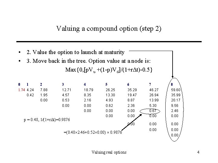
Valuing a compound option (step 2) • 2. Value the option to launch at maturity • 3. Move back in the tree. Option value at a node is: Max{0, [p. Vu +(1 -p)Vd]/(1+r t)-0. 5} 0 1 1. 74 4. 24 0. 42 2 7. 88 1. 95 0. 00 3 12. 71 4. 57 0. 53 0. 00 p = 0. 48, 1/(1+r t)=0. 9876 4 18. 79 8. 35 2. 16 0. 00 5 26. 25 13. 30 4. 93 0. 62 0. 00 =(0. 48 2. 46+0. 52 0. 00) 0. 9876 Valuing real options 6 35. 29 19. 47 8. 87 2. 36 0. 00 7 46. 27 26. 94 13. 99 5. 30 0. 67 0. 00 8 59. 60 35. 99 20. 17 9. 56 2. 46 0. 00 0. 00 4

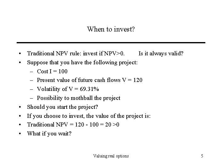
When to invest? • Traditional NPV rule: invest if NPV>0. Is it always valid? • Suppose that you have the following project: – Cost I = 100 – Present value of future cash flows V = 120 – Volatility of V = 69. 31% – Possibility to mothball the project • Should you start the project? • If you choose to invest, the value of the project is: • Traditional NPV = 120 - 100 = 20 >0 • What if you wait? Valuing real options 5

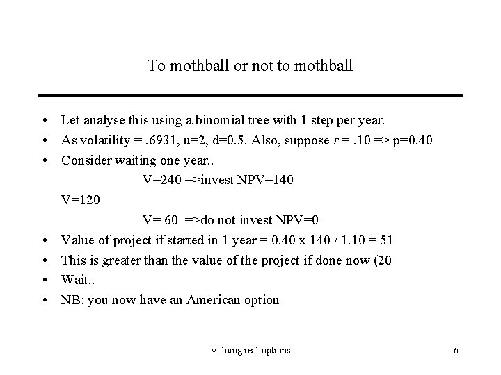
To mothball or not to mothball • Let analyse this using a binomial tree with 1 step per year. • As volatility =. 6931, u=2, d=0. 5. Also, suppose r =. 10 => p=0. 40 • Consider waiting one year. . V=240 =>invest NPV=140 V=120 V= 60 =>do not invest NPV=0 • Value of project if started in 1 year = 0. 40 x 140 / 1. 10 = 51 • This is greater than the value of the project if done now (20 • Wait. . • NB: you now have an American option Valuing real options 6

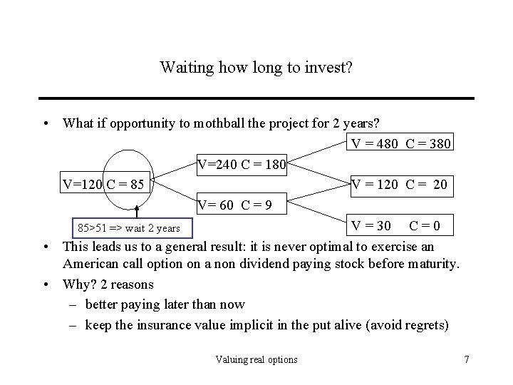
Waiting how long to invest? • What if opportunity to mothball the project for 2 years? V = 480 C = 380 V=240 C = 180 V=120 C = 85 V = 120 C = 20 V= 60 C = 9 V = 30 C = 0 85>51 => wait 2 years • This leads us to a general result: it is never optimal to exercise an American call option on a non dividend paying stock before maturity. • Why? 2 reasons – better paying later than now – keep the insurance value implicit in the put alive (avoid regrets) Valuing real options 7

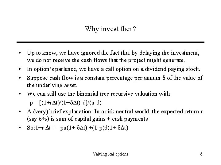
Why invest then? • Up to know, we have ignored the fact that by delaying the investment, we do not receive the cash flows that the project might generate. • In option’s parlance, we have a call option on a dividend paying stock. • Suppose cash flow is a constant percentage per annum of the value of the underlying asset. • We can still use the binomial tree recursive valuation with: p = [(1+r t)/(1+ t)-d]/(u-d) • A (very) brief explanation: In a risk neutral world, the expected return r (say 6%) is sum of capital gains + cash payments • So: 1+r t = pu(1+ t) +(1 -p)d(1+ t) Valuing real options 8

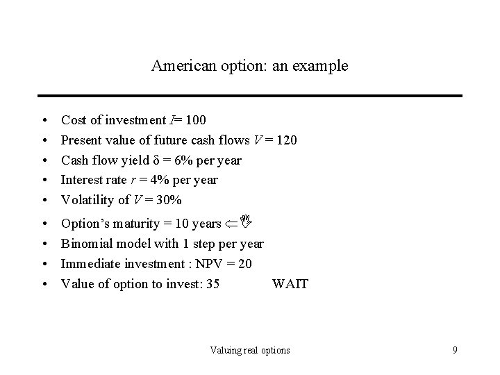
American option: an example • • • Cost of investment I= 100 Present value of future cash flows V = 120 Cash flow yield = 6% per year Interest rate r = 4% per year Volatility of V = 30% • • Option’s maturity = 10 years Binomial model with 1 step per year Immediate investment : NPV = 20 Value of option to invest: 35 WAIT Valuing real options 9

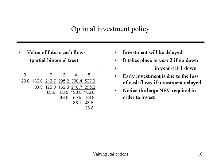
Optimal investment policy • Value of future cash flows (partial binomial tree) 0 1 2 3 120. 0 162. 0 218. 7 295. 2 88. 9 120. 0 162. 0 65. 9 88. 9 48. 8 4 398. 4 218. 7 120. 0 65. 9 36. 1 5 537. 8 295. 2 162. 0 88. 9 48. 8 26. 8 • • • Investment will be delayed. It takes place in year 2 if no down in year 4 if 1 down Early investment is due to the loss of cash flows if investment delayed. Notice the large NPV required in order to invest Valuing real options 10

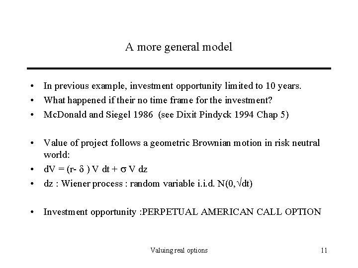
A more general model • In previous example, investment opportunity limited to 10 years. • What happened if their no time frame for the investment? • Mc. Donald and Siegel 1986 (see Dixit Pindyck 1994 Chap 5) • Value of project follows a geometric Brownian motion in risk neutral world: • d. V = (r- ) V dt + V dz • dz : Wiener process : random variable i. i. d. N(0, dt) • Investment opportunity : PERPETUAL AMERICAN CALL OPTION Valuing real options 11

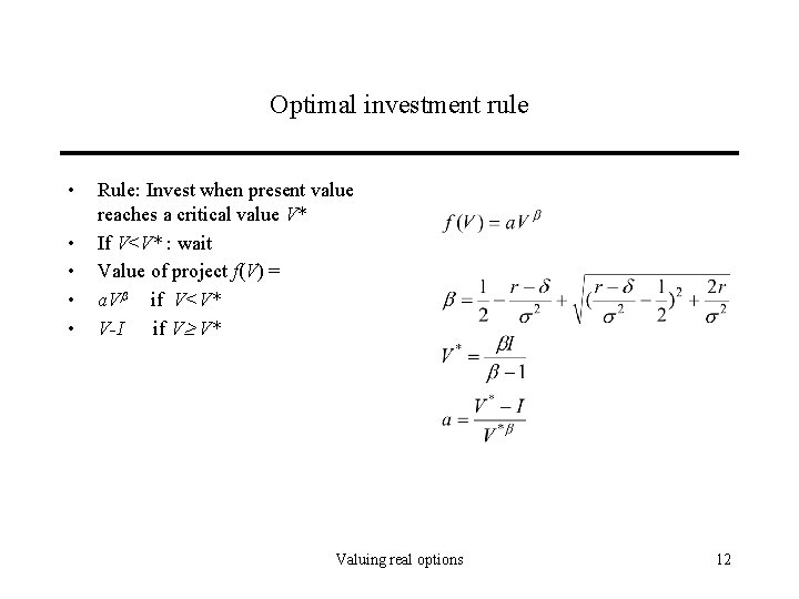
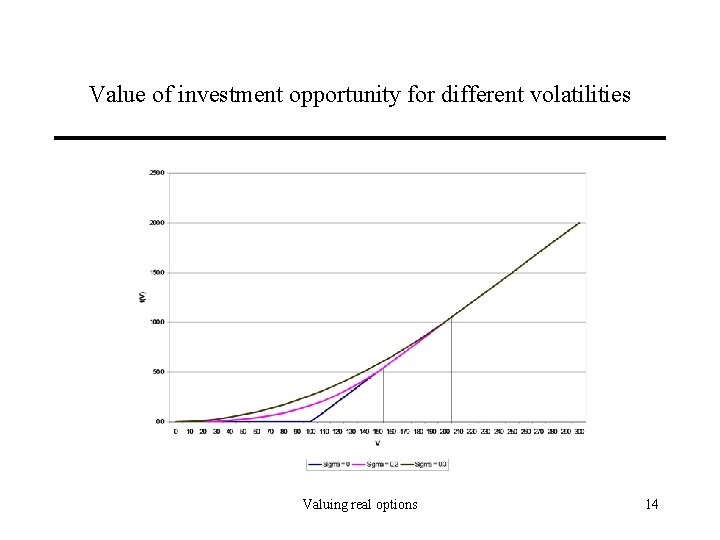
Optimal investment rule • • • Rule: Invest when present value reaches a critical value V* If V<V* : wait Value of project f(V) = a. V if V<V* V-I if V V* Valuing real options 12

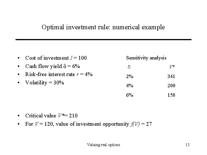
Optimal investment rule: numerical example • • Cost of investment I = 100 Cash flow yield = 6% Risk-free interest rate r = 4% Volatility = 30% Sensitivity analysis V* 2% 341 4% 200 6% 158 • Critical value V*= 210 • For V = 120, value of investment opportunity f(V) = 27 Valuing real options 13

Value of investment opportunity for different volatilities Valuing real options 14