Chapter 13 Comparing Several Means OneWay ANOVA January

Chapter 13: Comparing Several Means (One-Way ANOVA) January 22 1

In Chapter 13: 13. 1 Descriptive Statistics 13. 2 The Problem of Multiple Comparisons 13. 3 Analysis of Variance 13. 4 Post Hoc Comparisons 13. 5 The Equal Variance Assumption 13. 6 Introduction to Nonparametric Tests

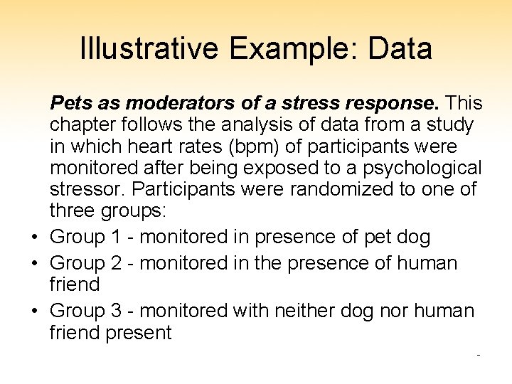
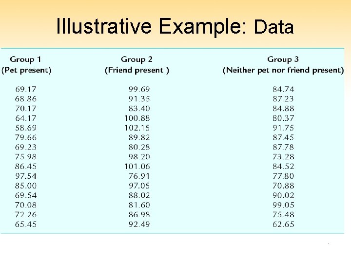
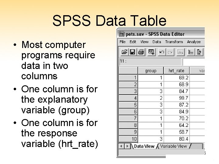
Illustrative Example: Data Pets as moderators of a stress response. This chapter follows the analysis of data from a study in which heart rates (bpm) of participants were monitored after being exposed to a psychological stressor. Participants were randomized to one of three groups: • Group 1 - monitored in presence of pet dog • Group 2 - monitored in the presence of human friend • Group 3 - monitored with neither dog nor human friend present 3

Illustrative Example: Data 4

SPSS Data Table • Most computer programs require data in two columns • One column is for the explanatory variable (group) • One column is for the response variable (hrt_rate) 5

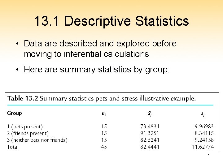
13. 1 Descriptive Statistics • Data are described and explored before moving to inferential calculations • Here are summary statistics by group: 6

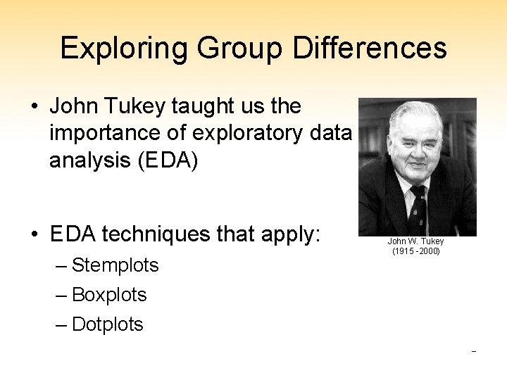
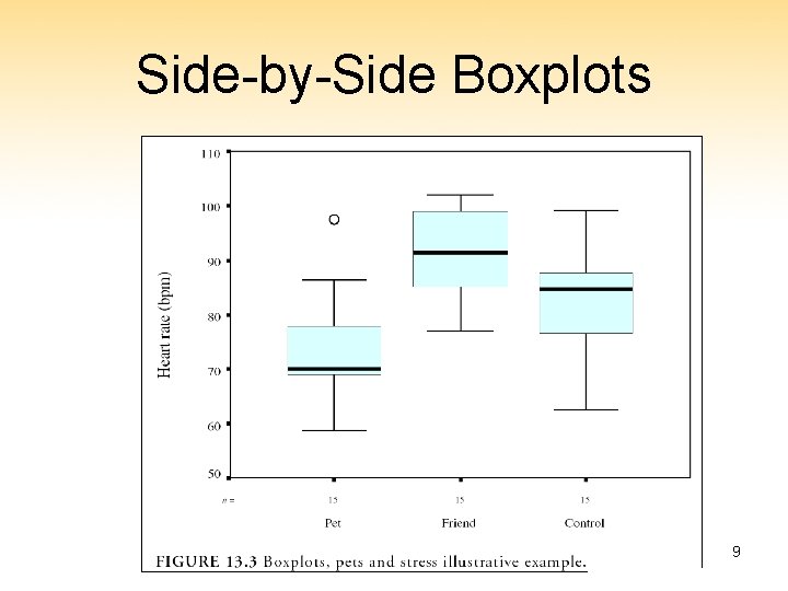
Exploring Group Differences • John Tukey taught us the importance of exploratory data analysis (EDA) • EDA techniques that apply: – Stemplots – Boxplots – Dotplots John W. Tukey (1915 -2000) 7

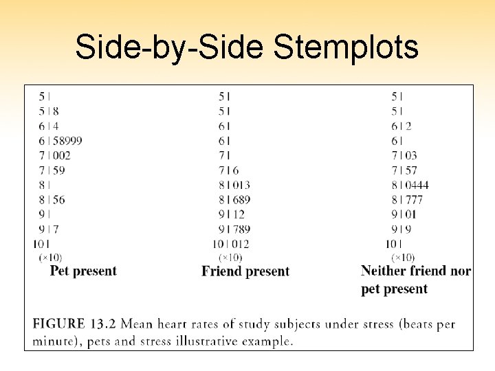
Side-by-Side Stemplots 8

Side-by-Side Boxplots 9

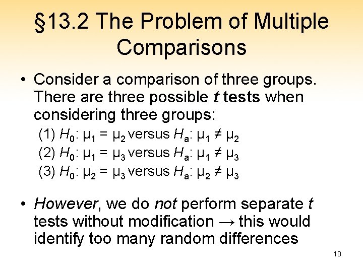
§ 13. 2 The Problem of Multiple Comparisons • Consider a comparison of three groups. There are three possible t tests when considering three groups: (1) H 0: μ 1 = μ 2 versus Ha: μ 1 ≠ μ 2 (2) H 0: μ 1 = μ 3 versus Ha: μ 1 ≠ μ 3 (3) H 0: μ 2 = μ 3 versus Ha: μ 2 ≠ μ 3 • However, we do not perform separate t tests without modification → this would identify too many random differences 10

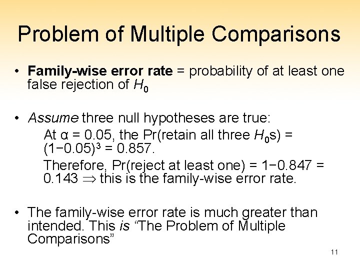
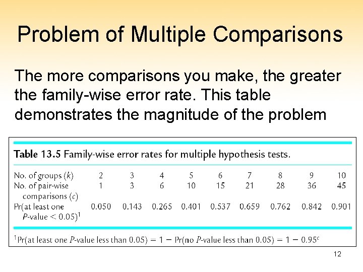
Problem of Multiple Comparisons • Family-wise error rate = probability of at least one false rejection of H 0 • Assume three null hypotheses are true: At α = 0. 05, the Pr(retain all three H 0 s) = (1− 0. 05)3 = 0. 857. Therefore, Pr(reject at least one) = 1− 0. 847 = 0. 143 this is the family-wise error rate. • The family-wise error rate is much greater than intended. This is “The Problem of Multiple Comparisons” 11

Problem of Multiple Comparisons The more comparisons you make, the greater the family-wise error rate. This table demonstrates the magnitude of the problem 12

Mitigating the Problem of Multiple Comparisons Two-step approach: 1. Test for overall significance using a technique called “Analysis of Variance” 2. Do post hoc comparison on individual groups 13

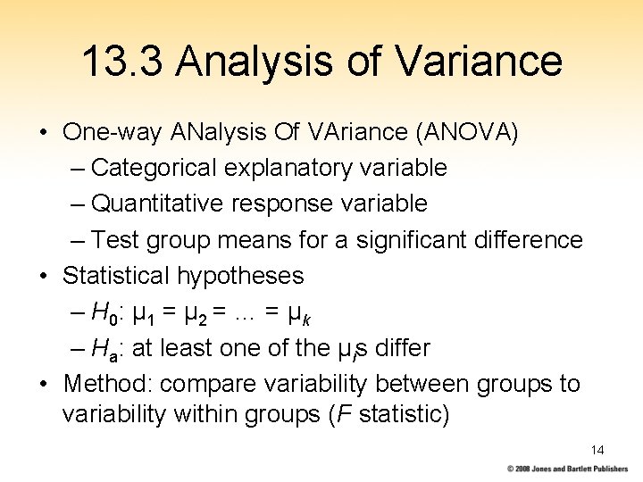
13. 3 Analysis of Variance • One-way ANalysis Of VAriance (ANOVA) – Categorical explanatory variable – Quantitative response variable – Test group means for a significant difference • Statistical hypotheses – H 0: μ 1 = μ 2 = … = μ k – Ha: at least one of the μis differ • Method: compare variability between groups to variability within groups (F statistic) 14

Analysis of Variance Overview, cont. R. A. Fisher (1890 -1962) The F in the F statistic stands for “Fisher” 15

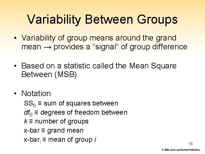
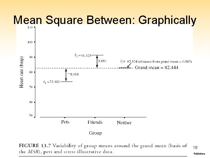
Variability Between Groups • Variability of group means around the grand mean → provides a “signal” of group difference • Based on a statistic called the Mean Square Between (MSB) • Notation SSB ≡ sum of squares between df. B ≡ degrees of freedom between k ≡ number of groups x-bar ≡ grand mean x-bari ≡ mean of group i 16

Mean Square Between: Formula • Sum of Squares Between [Groups] • Degrees of Freedom Between • Mean Square Between 17

Mean Square Between: Graphically 18

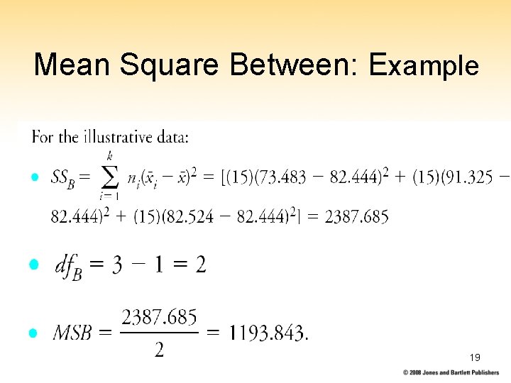
Mean Square Between: Example 19

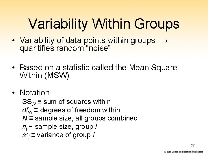
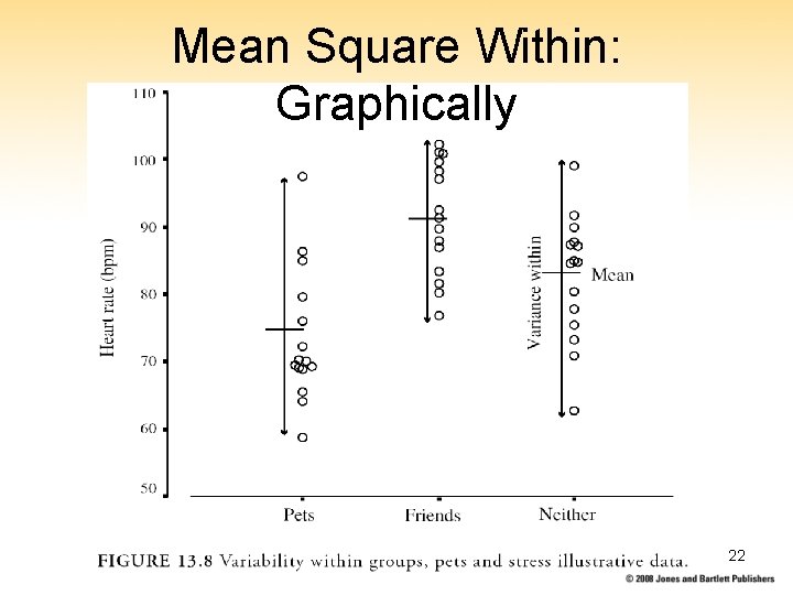
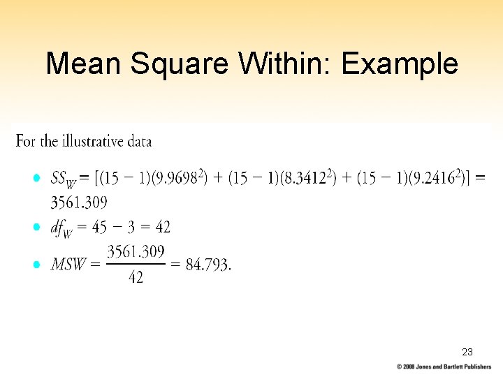
Variability Within Groups • Variability of data points within groups → quantifies random “noise” • Based on a statistic called the Mean Square Within (MSW) • Notation SSW ≡ sum of squares within df. W ≡ degrees of freedom within N ≡ sample size, all groups combined ni ≡ sample size, group I s 2 i ≡ variance of group i 20

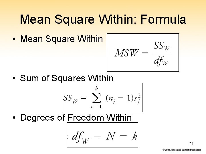
Mean Square Within: Formula • Mean Square Within • Sum of Squares Within • Degrees of Freedom Within 21

Mean Square Within: Graphically 22

Mean Square Within: Example 23

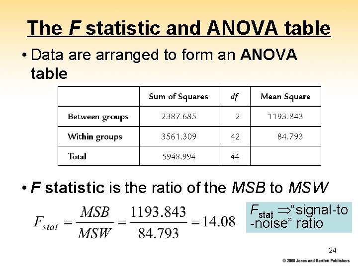
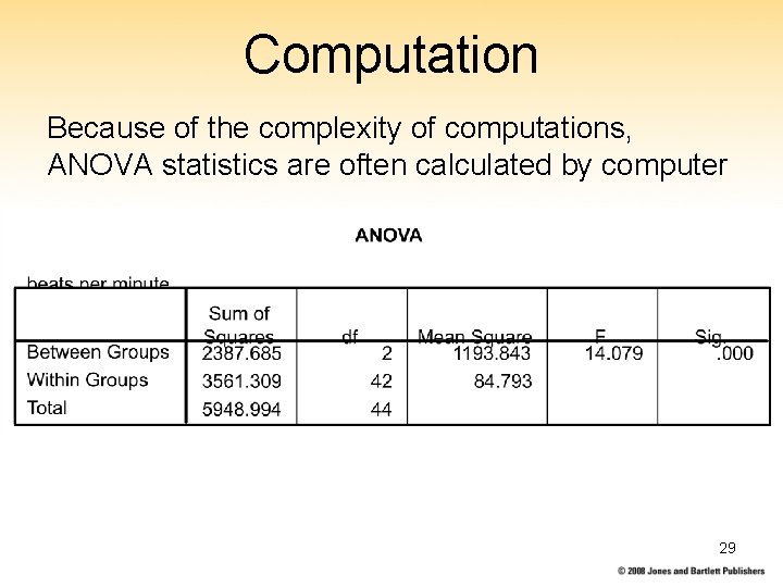
The F statistic and ANOVA table • Data are arranged to form an ANOVA table • F statistic is the ratio of the MSB to MSW Fstat “signal-to -noise” ratio 24

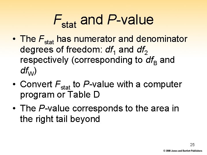
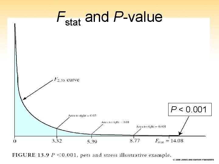
Fstat and P-value • The Fstat has numerator and denominator degrees of freedom: df 1 and df 2 respectively (corresponding to df. B and df. W) • Convert Fstat to P-value with a computer program or Table D • The P-value corresponds to the area in the right tail beyond 25

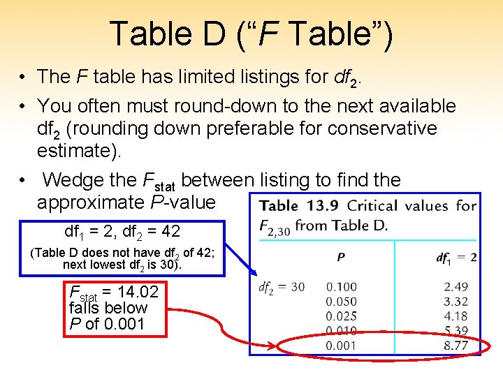
Table D (“F Table”) • The F table has limited listings for df 2. • You often must round-down to the next available df 2 (rounding down preferable for conservative estimate). • Wedge the Fstat between listing to find the approximate P-value df 1 = 2, df 2 = 42 (Table D does not have df 2 of 42; next lowest df 2 is 30). Fstat = 14. 02 falls below P of 0. 001 26

Fstat and P-value P < 0. 001 27

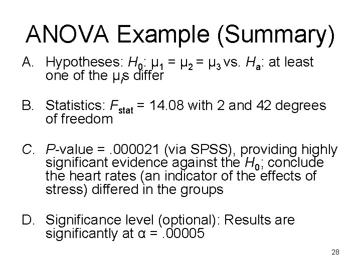
ANOVA Example (Summary) A. Hypotheses: H 0: μ 1 = μ 2 = μ 3 vs. Ha: at least one of the μis differ B. Statistics: Fstat = 14. 08 with 2 and 42 degrees of freedom C. P-value =. 000021 (via SPSS), providing highly significant evidence against the H 0; conclude the heart rates (an indicator of the effects of stress) differed in the groups D. Significance level (optional): Results are significantly at α =. 00005 28

Computation Because of the complexity of computations, ANOVA statistics are often calculated by computer 29

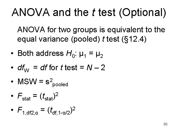
ANOVA and the t test (Optional) ANOVA for two groups is equivalent to the equal variance (pooled) t test (§ 12. 4) • Both address H 0: μ 1 = μ 2 • df. W = df for t test = N – 2 • MSW = s 2 pooled • Fstat = (tstat)2 • F 1, df 2, α = (tdf, 1 -α/2)2 30

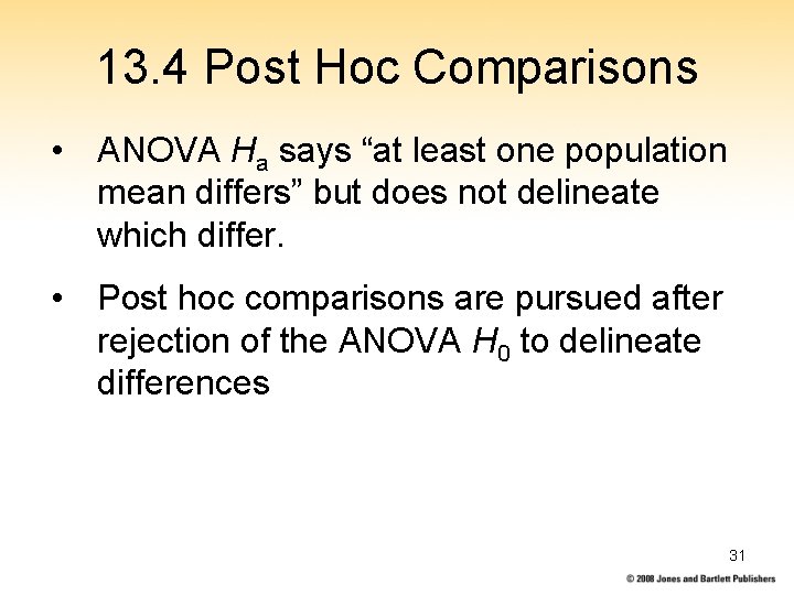
13. 4 Post Hoc Comparisons • ANOVA Ha says “at least one population mean differs” but does not delineate which differ. • Post hoc comparisons are pursued after rejection of the ANOVA H 0 to delineate differences 31

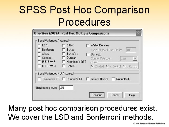
SPSS Post Hoc Comparison Procedures Many post hoc comparison procedures exist. We cover the LSD and Bonferroni methods. 32

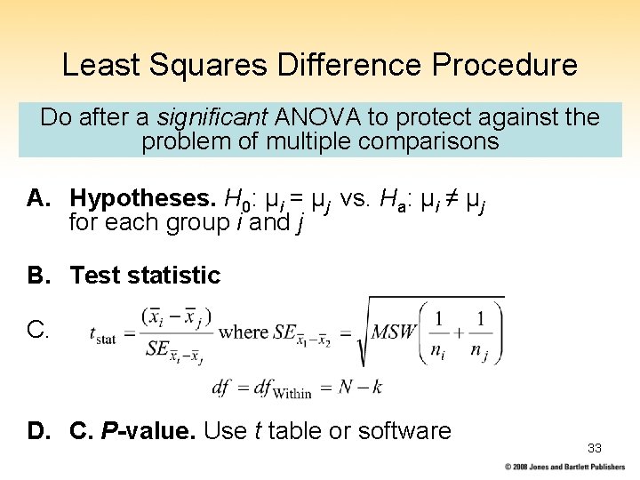
Least Squares Difference Procedure Do after a significant ANOVA to protect against the problem of multiple comparisons A. Hypotheses. H 0: μi = μj vs. Ha: μi ≠ μj for each group i and j B. Test statistic C. D. C. P-value. Use t table or software 33

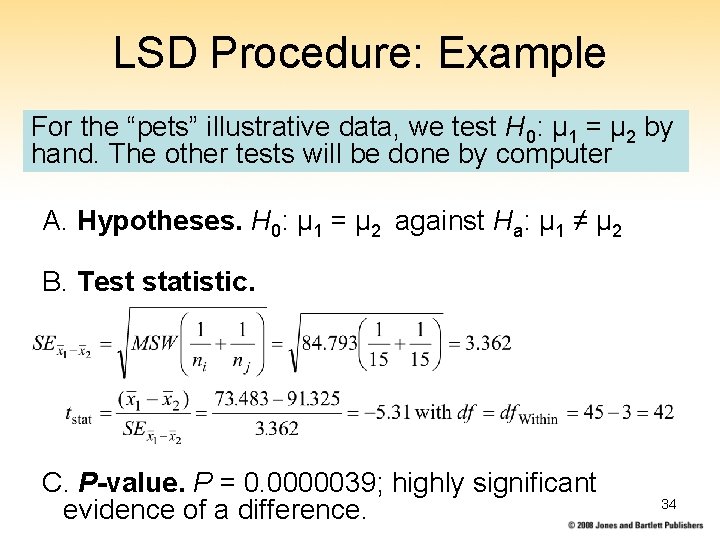
LSD Procedure: Example For the “pets” illustrative data, we test H 0: μ 1 = μ 2 by hand. The other tests will be done by computer A. Hypotheses. H 0: μ 1 = μ 2 against Ha: μ 1 ≠ μ 2 B. Test statistic. C. P-value. P = 0. 0000039; highly significant evidence of a difference. 34

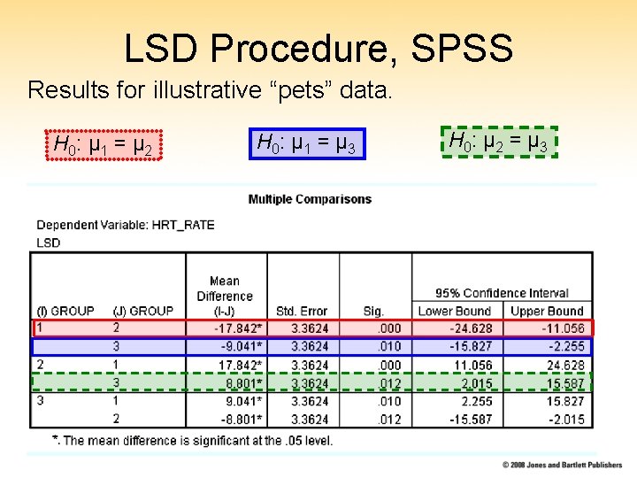
LSD Procedure, SPSS Results for illustrative “pets” data. H 0: μ 1 = μ 2 H 0: μ 1 = μ 3 H 0: μ 2 = μ 3 35

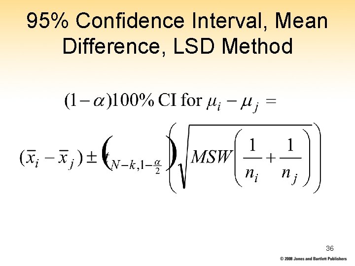
95% Confidence Interval, Mean Difference, LSD Method 36

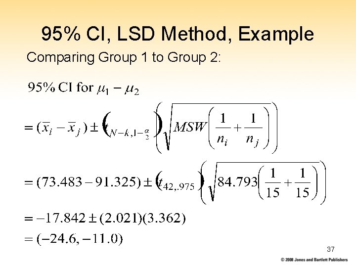
95% CI, LSD Method, Example Comparing Group 1 to Group 2: 37

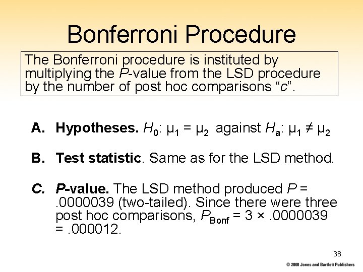
Bonferroni Procedure The Bonferroni procedure is instituted by multiplying the P-value from the LSD procedure by the number of post hoc comparisons “c”. A. Hypotheses. H 0: μ 1 = μ 2 against Ha: μ 1 ≠ μ 2 B. Test statistic. Same as for the LSD method. C. P-value. The LSD method produced P =. 0000039 (two-tailed). Since there were three post hoc comparisons, PBonf = 3 ×. 0000039 =. 000012. 38

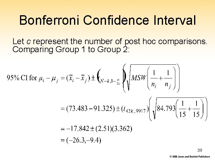
Bonferroni Confidence Interval Let c represent the number of post hoc comparisons. Comparing Group 1 to Group 2: 39

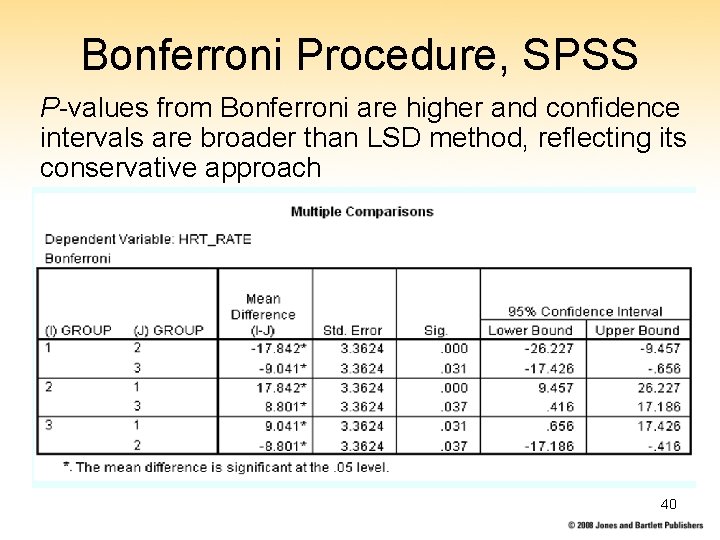
Bonferroni Procedure, SPSS P-values from Bonferroni are higher and confidence intervals are broader than LSD method, reflecting its conservative approach 40

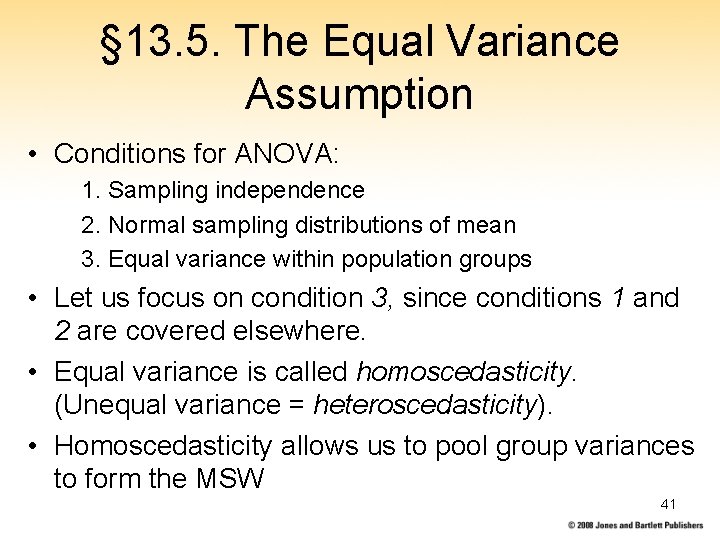
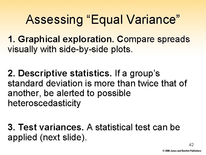
§ 13. 5. The Equal Variance Assumption • Conditions for ANOVA: 1. Sampling independence 2. Normal sampling distributions of mean 3. Equal variance within population groups • Let us focus on condition 3, since conditions 1 and 2 are covered elsewhere. • Equal variance is called homoscedasticity. (Unequal variance = heteroscedasticity). • Homoscedasticity allows us to pool group variances to form the MSW 41

Assessing “Equal Variance” 1. Graphical exploration. Compare spreads visually with side-by-side plots. 2. Descriptive statistics. If a group’s standard deviation is more than twice that of another, be alerted to possible heteroscedasticity 3. Test variances. A statistical test can be applied (next slide). 42

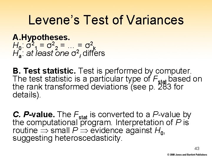
Levene’s Test of Variances A. Hypotheses. H 0: σ 21 = σ 22 = … = σ 2 k Ha: at least one σ2 i differs B. Test statistic. Test is performed by computer. The test statistic is a particular type of Fstat based on the rank transformed deviations (see p. 283 for details). C. P-value. The Fstat is converted to a P-value by the computational program. Interpretation of P is routine small P evidence against H 0, suggesting heteroscedasticity. 43

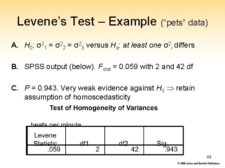
Levene’s Test – Example (“pets” data) A. H 0: σ21 = σ22 = σ23 versus Ha: at least one σ2 i differs B. SPSS output (below). Fstat = 0. 059 with 2 and 42 df C. P = 0. 943. Very weak evidence against H 0 retain assumption of homoscedasticity 44

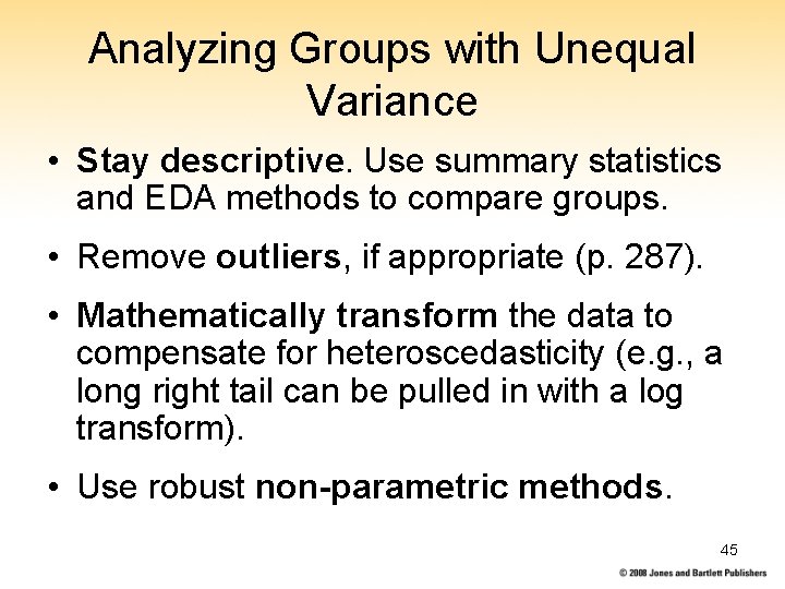
Analyzing Groups with Unequal Variance • Stay descriptive. Use summary statistics and EDA methods to compare groups. • Remove outliers, if appropriate (p. 287). • Mathematically transform the data to compensate for heteroscedasticity (e. g. , a long right tail can be pulled in with a log transform). • Use robust non-parametric methods. 45

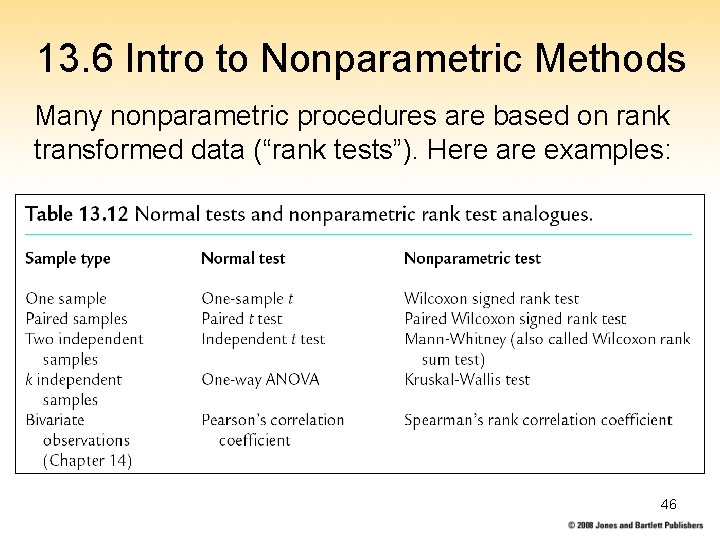
13. 6 Intro to Nonparametric Methods Many nonparametric procedures are based on rank transformed data (“rank tests”). Here are examples: 46

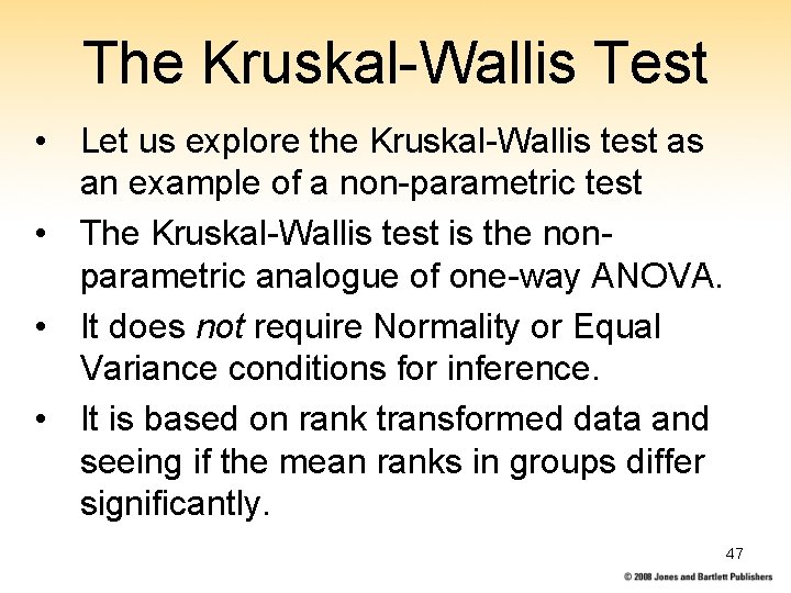
The Kruskal-Wallis Test • Let us explore the Kruskal-Wallis test as an example of a non-parametric test • The Kruskal-Wallis test is the nonparametric analogue of one-way ANOVA. • It does not require Normality or Equal Variance conditions for inference. • It is based on rank transformed data and seeing if the mean ranks in groups differ significantly. 47

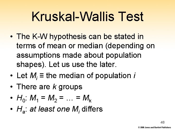
Kruskal-Wallis Test • The K-W hypothesis can be stated in terms of mean or median (depending on assumptions made about population shapes). Let us use the later. • Let Mi ≡ the median of population i • There are k groups • H 0 : M 1 = M 2 = … = Mk • Ha: at least one Mi differs 48

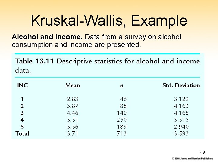
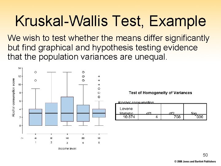
Kruskal-Wallis, Example Alcohol and income. Data from a survey on alcohol consumption and income are presented. 49

Kruskal-Wallis Test, Example We wish to test whether the means differ significantly but find graphical and hypothesis testing evidence that the population variances are unequal. 50

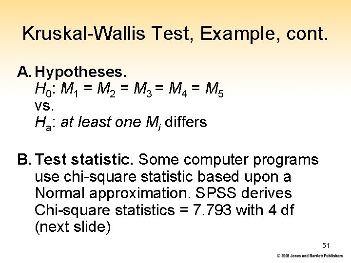
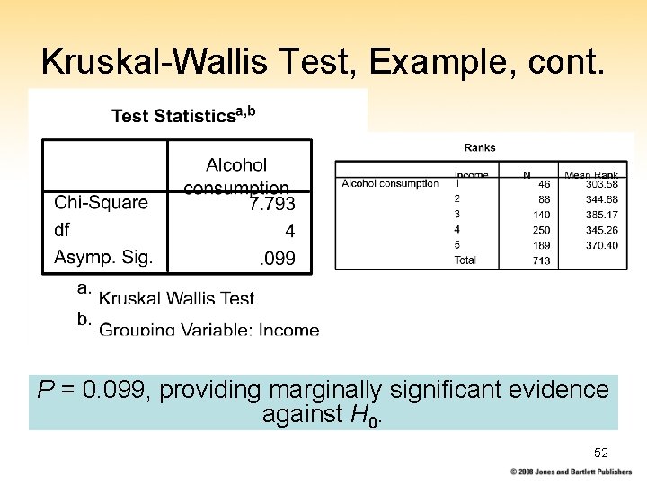
Kruskal-Wallis Test, Example, cont. A. Hypotheses. H 0 : M 1 = M 2 = M 3 = M 4 = M 5 vs. Ha: at least one Mi differs B. Test statistic. Some computer programs use chi-square statistic based upon a Normal approximation. SPSS derives Chi-square statistics = 7. 793 with 4 df (next slide) 51

Kruskal-Wallis Test, Example, cont. P = 0. 099, providing marginally significant evidence against H 0. 52