CDA 6530 Performance Models of Computers and Networks

CDA 6530: Performance Models of Computers and Networks Chapter 4: Using Matlab for Performance Analysis and Simulation

Objective q Learn a useful tool for mathematical analysis and simulation q q q Interpreted language, easy to learn Use it to facilitate our simulation projects A good tool to plot simulation/experiment results figures for academic papers More powerful than excel q Could directly create. eps for Latex q 2

Introduction q q Mat. Lab : Matrix Laboratory Numerical Computations with matrices q q Every number can be represented as matrix Why Matlab? User Friendly (GUI) q Easy to work with q Powerful tools for complex mathematics q q Matlab has extensive demo and tutorials to learn by yourself q Use help command 3

Matlab Software Access q q all UCF in-campus computers have student-version Matlab installed If you have no access to Matlab, you can use Octave, an open-source free software q q http: //www. gnu. org/software/octave/ The programming should be almost identical 4

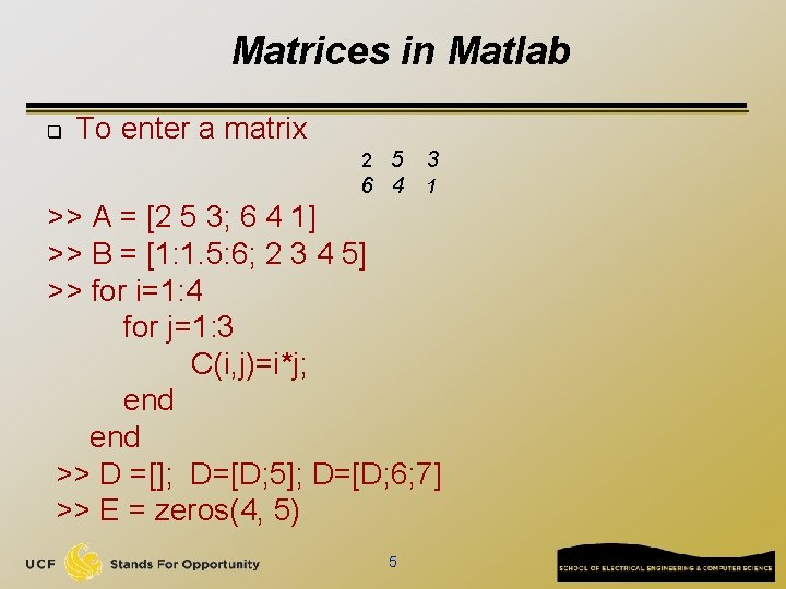
Matrices in Matlab q To enter a matrix 2 5 3 6 4 1 >> A = [2 5 3; 6 4 1] >> B = [1: 1. 5: 6; 2 3 4 5] >> for i=1: 4 for j=1: 3 C(i, j)=i*j; end >> D =[]; D=[D; 5]; D=[D; 6; 7] >> E = zeros(4, 5) 5

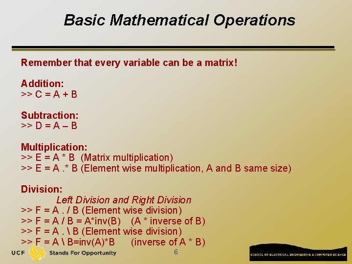
Basic Mathematical Operations Remember that every variable can be a matrix! Addition: >> C = A + B Subtraction: >> D = A – B Multiplication: >> E = A * B (Matrix multiplication) >> E = A. * B (Element wise multiplication, A and B same size) Division: Left Division and Right Division >> F = A. / B (Element wise division) >> F = A / B = A*inv(B) (A * inverse of B) >> F = A. B (Element wise division) >> F = A B=inv(A)*B (inverse of A * B) 6

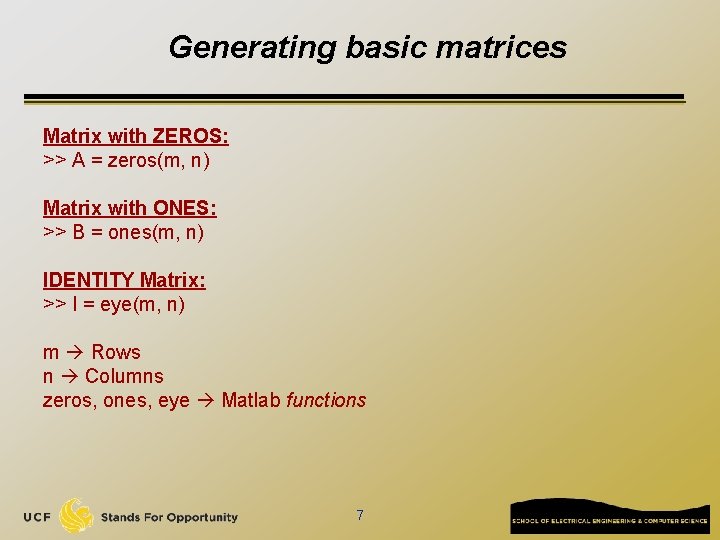
Generating basic matrices Matrix with ZEROS: >> A = zeros(m, n) Matrix with ONES: >> B = ones(m, n) IDENTITY Matrix: >> I = eye(m, n) m Rows n Columns zeros, ones, eye Matlab functions 7

Obtain Information q q Size(A): return [m n] Length(A): length of a vector q q B = A(2: 4, 3: 5) q q Length(A) = max(size(A)) B is the subset of A from row 2 to row 4, column 3 to column 5 A(: , 2)=[] q Delete second column 8

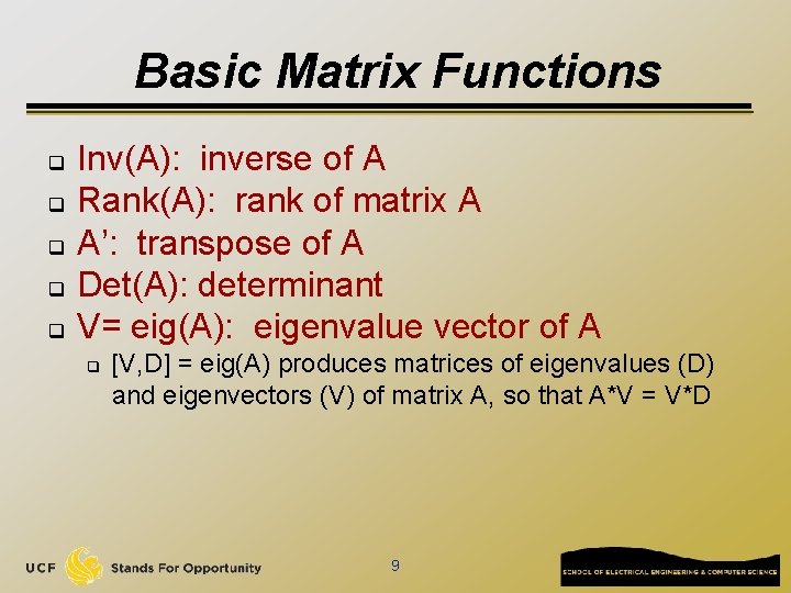
Basic Matrix Functions q q q Inv(A): inverse of A Rank(A): rank of matrix A A’: transpose of A Det(A): determinant V= eig(A): eigenvalue vector of A q [V, D] = eig(A) produces matrices of eigenvalues (D) and eigenvectors (V) of matrix A, so that A*V = V*D 9

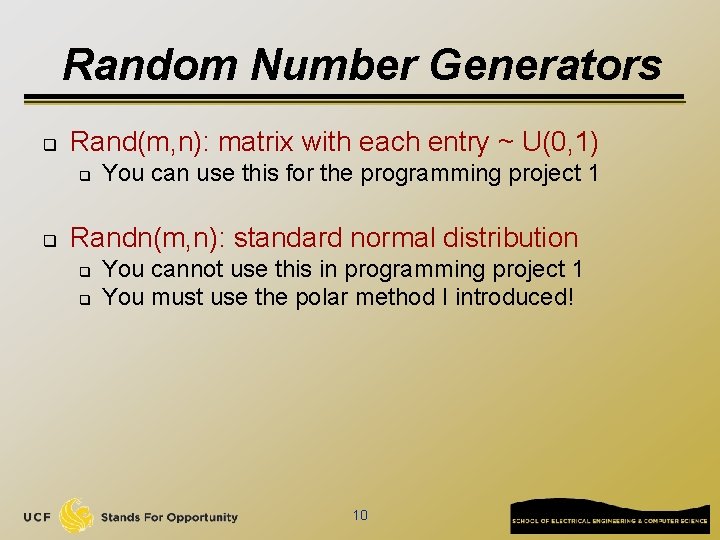
Random Number Generators q Rand(m, n): matrix with each entry ~ U(0, 1) q q You can use this for the programming project 1 Randn(m, n): standard normal distribution q q You cannot use this in programming project 1 You must use the polar method I introduced! 10

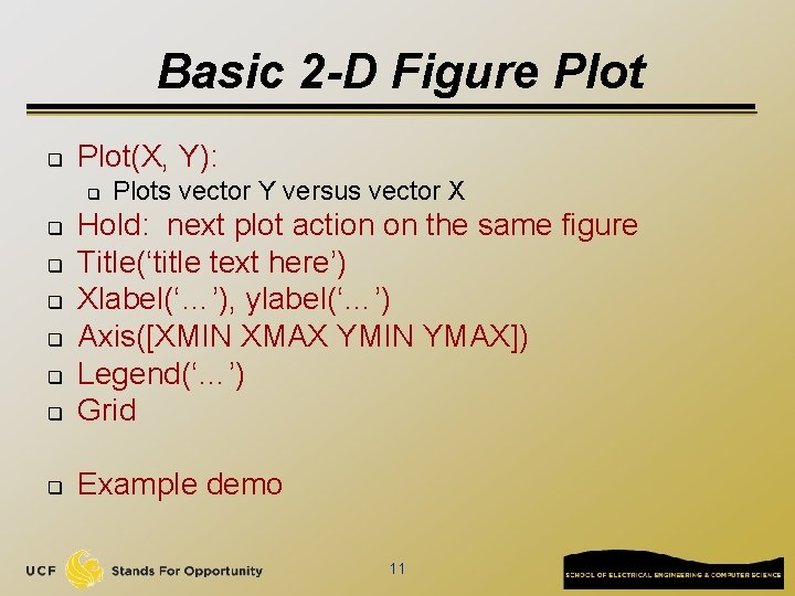
Basic 2 -D Figure Plot q Plot(X, Y): q Plots vector Y versus vector X q Hold: next plot action on the same figure Title(‘title text here’) Xlabel(‘…’), ylabel(‘…’) Axis([XMIN XMAX YMIN YMAX]) Legend(‘…’) Grid q Example demo q q q 11

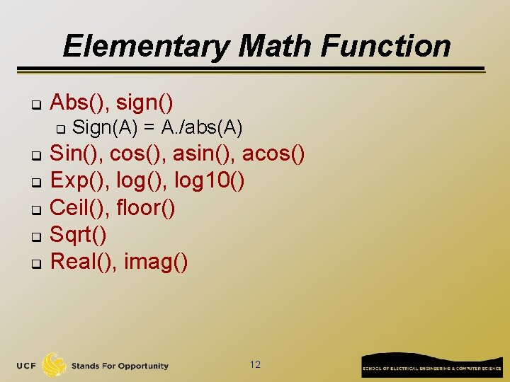
Elementary Math Function q Abs(), sign() q q q Sign(A) = A. /abs(A) Sin(), cos(), asin(), acos() Exp(), log 10() Ceil(), floor() Sqrt() Real(), imag() 12

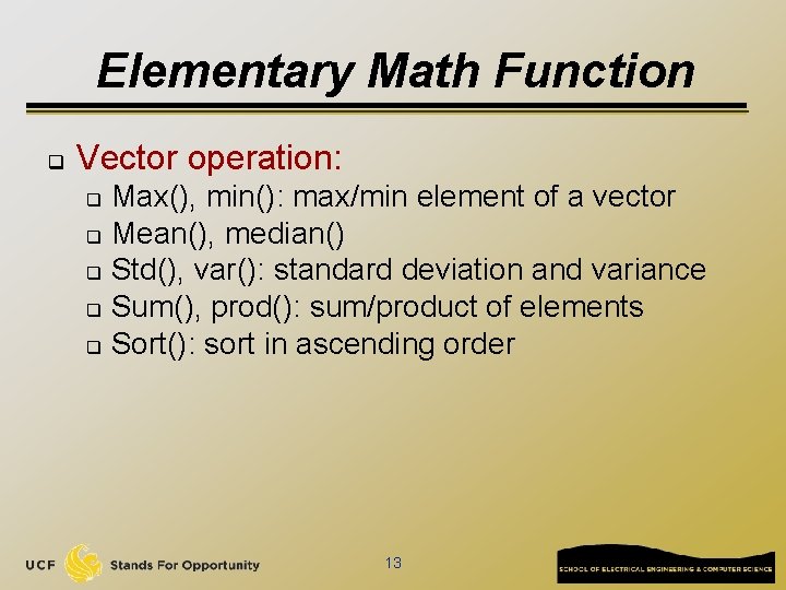
Elementary Math Function q Vector operation: Max(), min(): max/min element of a vector q Mean(), median() q Std(), var(): standard deviation and variance q Sum(), prod(): sum/product of elements q Sort(): sort in ascending order q 13

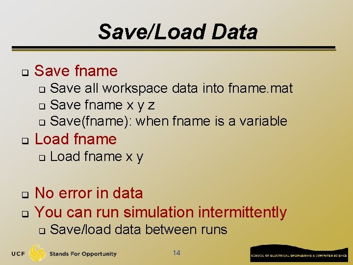
Save/Load Data q Save fname Save all workspace data into fname. mat q Save fname x y z q Save(fname): when fname is a variable q q Load fname q q q Load fname x y No error in data You can run simulation intermittently q Save/load data between runs 14

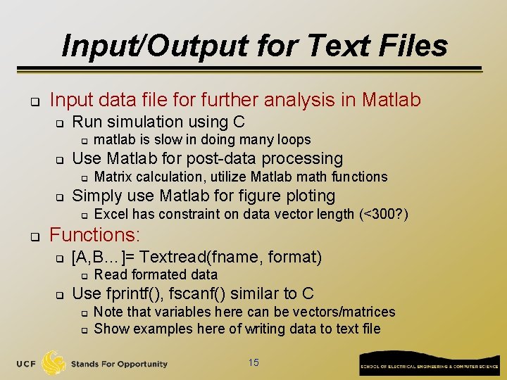
Input/Output for Text Files q Input data file for further analysis in Matlab q Run simulation using C q q Use Matlab for post-data processing q q Matrix calculation, utilize Matlab math functions Simply use Matlab for figure ploting q q matlab is slow in doing many loops Excel has constraint on data vector length (<300? ) Functions: q [A, B…]= Textread(fname, format) q q Read formated data Use fprintf(), fscanf() similar to C q q Note that variables here can be vectors/matrices Show examples here of writing data to text file 15

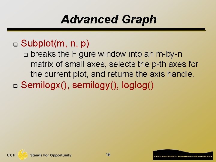
Advanced Graph q Subplot(m, n, p) q q breaks the Figure window into an m-by-n matrix of small axes, selects the p-th axes for the current plot, and returns the axis handle. Semilogx(), semilogy(), loglog() 16

3 -D plot q q x=[0: 10]; y=[0: 10]; z=x’*y; mesh(x, y, z); figure; surf(x, y, z); 17

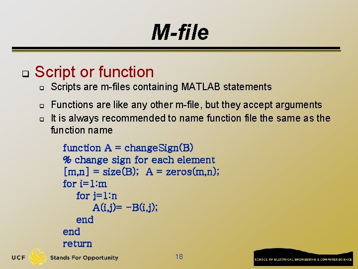
M-file q Script or function q q q Scripts are m-files containing MATLAB statements Functions are like any other m-file, but they accept arguments It is always recommended to name function file the same as the function name function A = change. Sign(B) % change sign for each element [m, n] = size(B); A = zeros(m, n); for i=1: m for j=1: n A(i, j)= -B(i, j); end return 18

Online Tutorials q q Matlab itself contains many tutorials Other online tutorials: http: //www. math. siu. edu/matlab/tutorials. html q http: //www. cs. cmu. edu/~ggordon/780/lecture s/matlab_tutorial. pdf q Google search “matlab tutorial ppt” to find a lot more q 19

Example on Using Matlab for Markov Chain Steady State Calculation 20

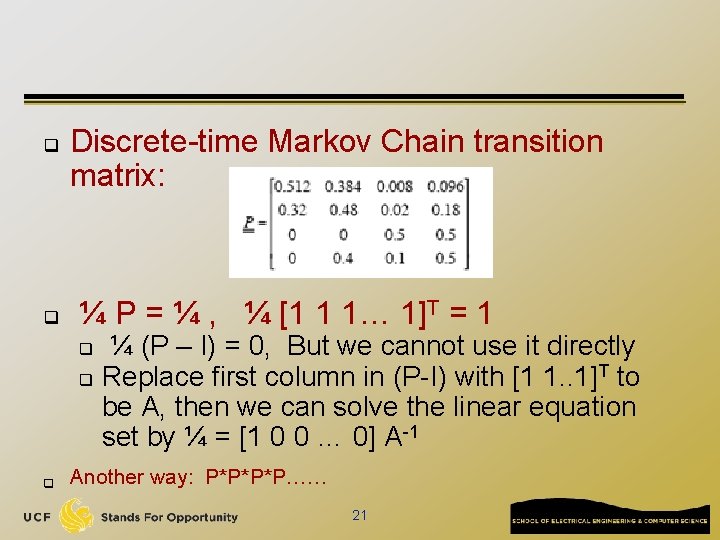
q q Discrete-time Markov Chain transition matrix: ¼ P = ¼ , ¼ [1 1 1… 1]T = 1 ¼ (P – I) = 0, But we cannot use it directly T q Replace first column in (P-I) with [1 1. . 1] to be A, then we can solve the linear equation set by ¼ = [1 0 0 … 0] A-1 q q Another way: P*P*P*P…… 21

Tutorial on Matlab Simulink 22

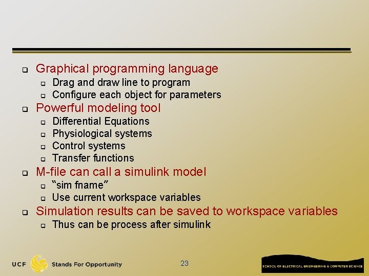
q Graphical programming language q q q Powerful modeling tool q q q Differential Equations Physiological systems Control systems Transfer functions M-file can call a simulink model q q q Drag and draw line to program Configure each object for parameters “sim fname” Use current workspace variables Simulation results can be saved to workspace variables q Thus can be process after simulink 23

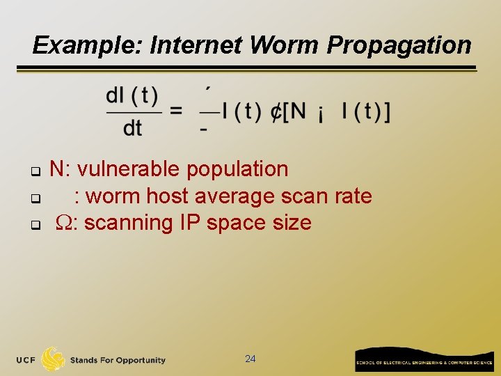
Example: Internet Worm Propagation q q q N: vulnerable population : worm host average scan rate : scanning IP space size 24

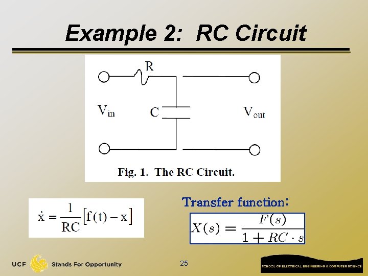
Example 2: RC Circuit Transfer function: 25

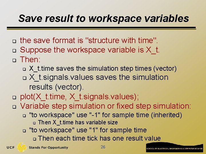
Save result to workspace variables q q q the save format is "structure with time". Suppose the workspace variable is X_t. Then: q X_t. time saves the simulation step times (vector) X_t. signals. values saves the simulation results (vector). plot(X_t. time, X_t. signals. values); Variable step simulation or fixed step simulation: q q "to workspace" use "-1" for sample time (inherited) q q Then X_t. time has variable size "to workspace" use "1" for sample time q Then each time tick has one result value 26