CDA 6530 Performance Models of Computers and Networks

CDA 6530: Performance Models of Computers and Networks Chapter 9: Statistical Simulation ---Discrete Event Simulation (DES)

Time Concept q physical time: time in the physical system q q simulation time: representation of physical time within the simulation q q q Noon, Oct. 14, 2008 to noon Nov. 1, 2008 floating point values in interval [0. 0, 17. 0] Example: 1. 5 represents one and half hour after physical system begins simulation wallclock time: time during the execution of the simulation, usually output from a hardware clock q 8: 00 to 10: 23 AM on Oct. 14, 2008 2

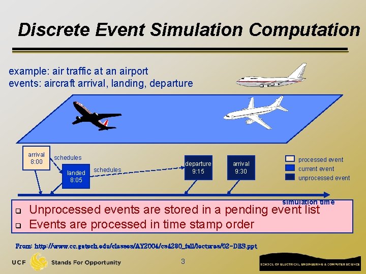
Discrete Event Simulation Computation example: air traffic at an airport events: aircraft arrival, landing, departure arrival 8: 00 schedules landed 8: 05 departure 9: 15 schedules arrival 9: 30 processed event current event unprocessed event simulation time q q Unprocessed events are stored in a pending event list Events are processed in time stamp order From: http: //www. cc. gatech. edu/classes/AY 2004/cs 4230_fall/lectures/02 -DES. ppt 3

DES: No Time Loop q Discrete event simulation has no time loop There are events that are scheduled. q At each run step, the next scheduled event with the lowest time schedule gets processed. q q The current time is then that time, the time when that event is supposed to occur. Accurate simulation compared to discretetime simulation Key: We have to keep the list of scheduled events sorted (in order) 4

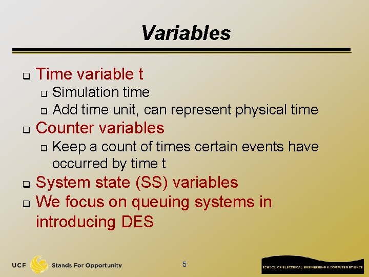
Variables q Time variable t Simulation time q Add time unit, can represent physical time q q Counter variables q q q Keep a count of times certain events have occurred by time t System state (SS) variables We focus on queuing systems in introducing DES 5

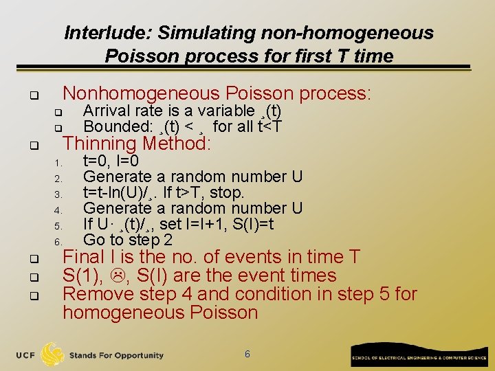
Interlude: Simulating non-homogeneous Poisson process for first T time Nonhomogeneous Poisson process: q q q Thinning Method: q 1. 2. 3. 4. 5. 6. q q q Arrival rate is a variable ¸(t) Bounded: ¸(t) < ¸ for all t<T t=0, I=0 Generate a random number U t=t-ln(U)/¸. If t>T, stop. Generate a random number U If U· ¸(t)/¸, set I=I+1, S(I)=t Go to step 2 Final I is the no. of events in time T S(1), , S(I) are the event times Remove step 4 and condition in step 5 for homogeneous Poisson 6

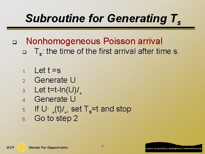
Subroutine for Generating Ts q Nonhomogeneous Poisson arrival q 1. 2. 3. 4. 5. 6. Ts: the time of the first arrival after time s. Let t =s Generate U Let t=t-ln(U)/¸ Generate U If U· ¸(t)/¸, set Ts=t and stop Go to step 2 7

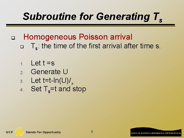
Subroutine for Generating Ts q Homogeneous Poisson arrival q 1. 2. 3. 4. Ts: the time of the first arrival after time s. Let t =s Generate U Let t=t-ln(U)/¸ Set Ts=t and stop 8

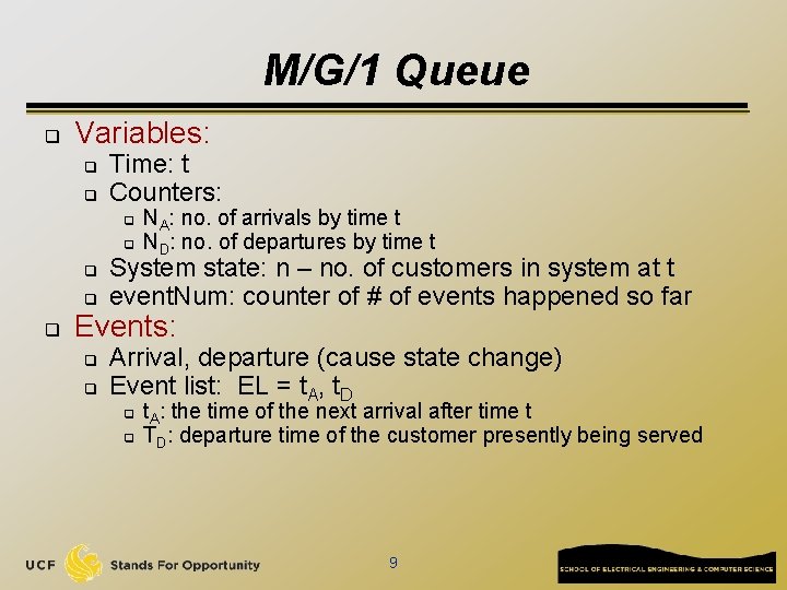
M/G/1 Queue q Variables: q q Time: t Counters: q q q NA: no. of arrivals by time t ND: no. of departures by time t System state: n – no. of customers in system at t event. Num: counter of # of events happened so far Events: q q Arrival, departure (cause state change) Event list: EL = t. A, t. D q q t. A: the time of the next arrival after time t TD: departure time of the customer presently being served 9

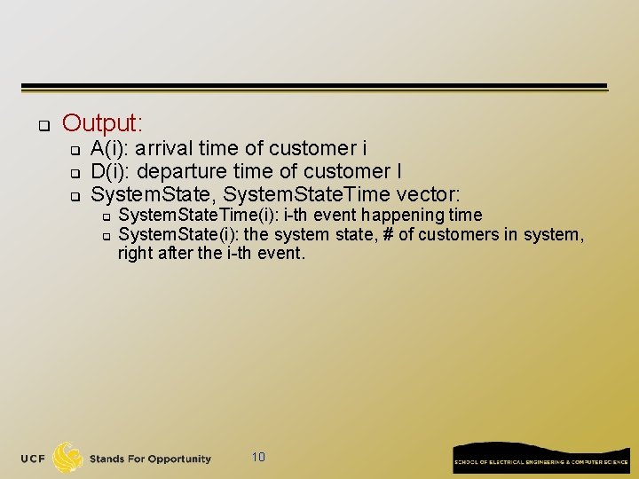
q Output: q q q A(i): arrival time of customer i D(i): departure time of customer I System. State, System. State. Time vector: q q System. State. Time(i): i-th event happening time System. State(i): the system state, # of customers in system, right after the i-th event. 10

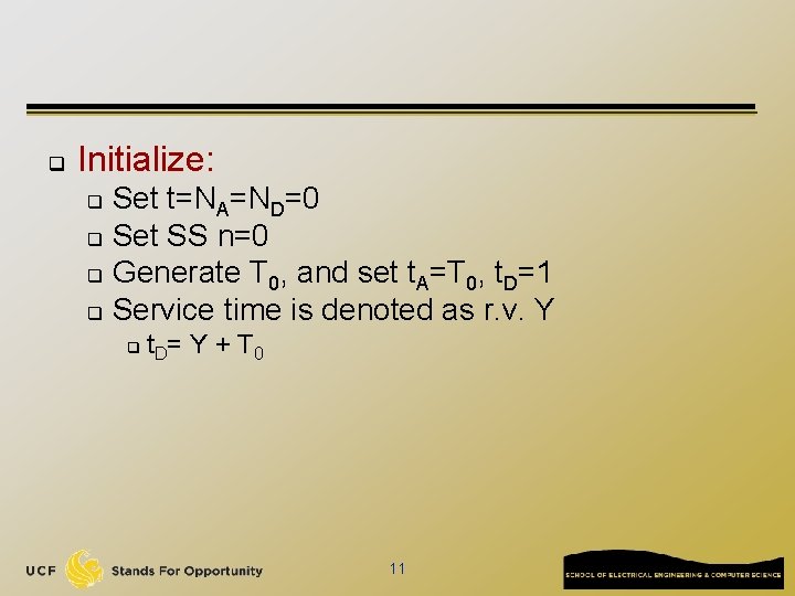
q Initialize: Set t=NA=ND=0 q Set SS n=0 q Generate T 0, and set t. A=T 0, t. D=1 q Service time is denoted as r. v. Y q t = Y + T 0 q D 11

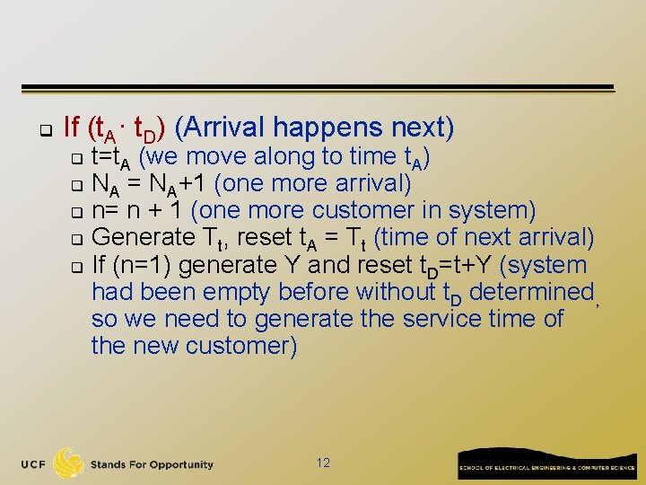
q If (t. A· t. D) (Arrival happens next) t=t. A (we move along to time t. A) q NA = NA+1 (one more arrival) q n= n + 1 (one more customer in system) q Generate Tt, reset t. A = Tt (time of next arrival) q If (n=1) generate Y and reset t. D=t+Y (system had been empty before without t. D determined, so we need to generate the service time of the new customer) q 12

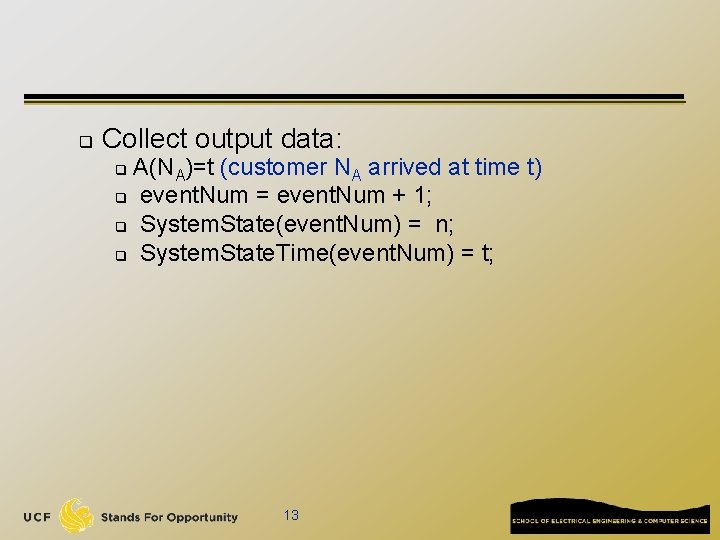
q Collect output data: A(NA)=t (customer NA arrived at time t) q event. Num = event. Num + 1; q System. State(event. Num) = n; q System. State. Time(event. Num) = t; q 13

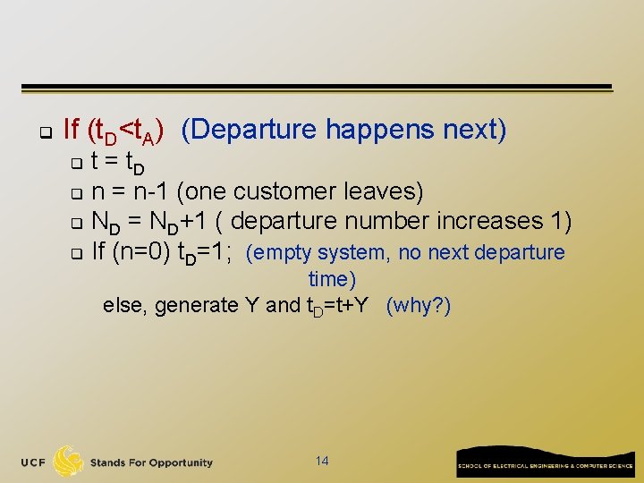
q If (t. D<t. A) (Departure happens next) t = t. D q n = n-1 (one customer leaves) q ND = ND+1 ( departure number increases 1) q If (n=0) t. D=1; (empty system, no next departure q time) else, generate Y and t. D=t+Y (why? ) 14

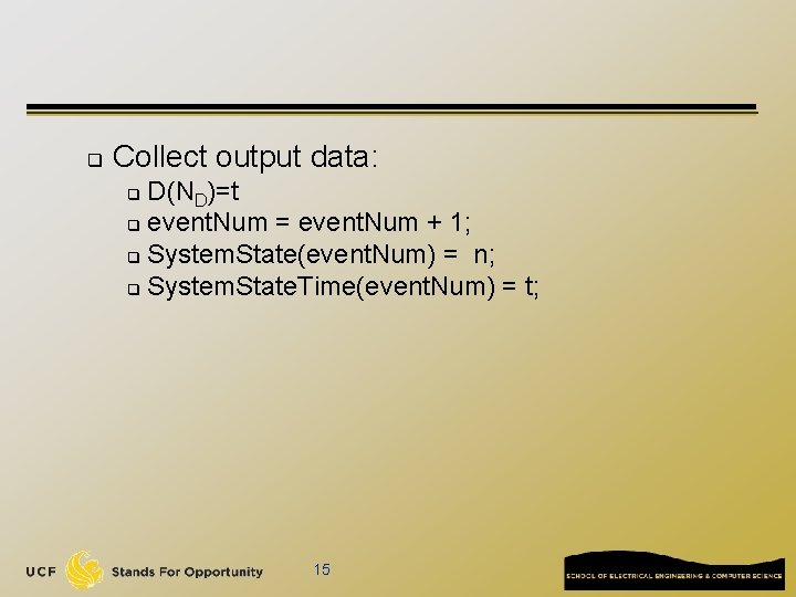
q Collect output data: D(ND)=t q event. Num = event. Num + 1; q System. State(event. Num) = n; q System. State. Time(event. Num) = t; q 15

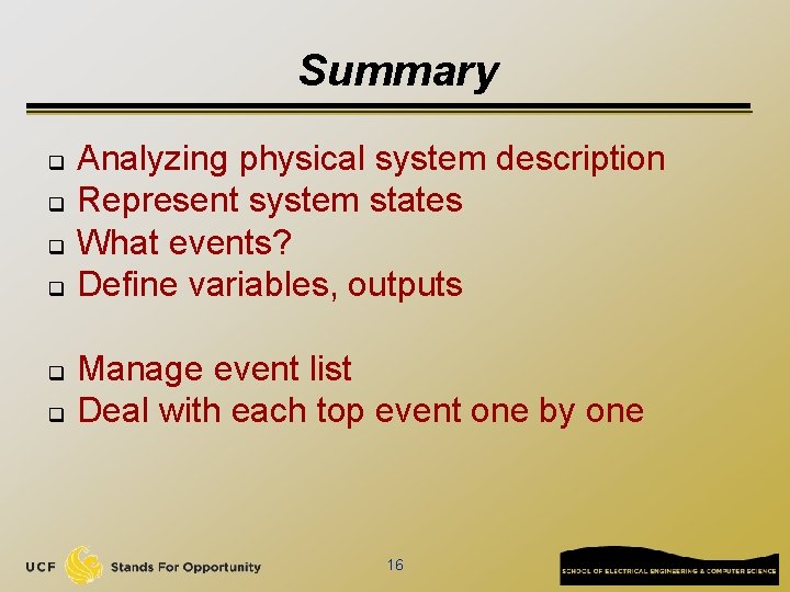
Summary q q q Analyzing physical system description Represent system states What events? Define variables, outputs Manage event list Deal with each top event one by one 16