CDA 6530 Performance Models of Computers and Networks

CDA 6530: Performance Models of Computers and Networks Chapter 8: Discrete Event Simulation Example --- Three callers problem in homwork 2

Problem Description q Two lines services three callers. Each caller makes calls that are exponentially distributed in length, with mean 1/¹. If both lines are in service by two callers and the third one requests service, the third caller will be blocked. A caller whose previous attempt to make a call was successful has an exponentially distributed time before attempting the next call, with rate ¸. A caller whose previous call attempt was blocked is impatient and tries to call again at twice that rate (2¸), also according to exponential distribution. The callers make their calls independent of one another. 2

Analysis Results q q 3 Steady state prob: ¼ Matlab code: Q = [………]; Pi = zeros(1, 6); Q_m = [Q(: , 1: 5) ones(6, 1)]; B = [0 0 0 1]; Pi = B * inv(Q_m);

Simulation based on Markov Model 4

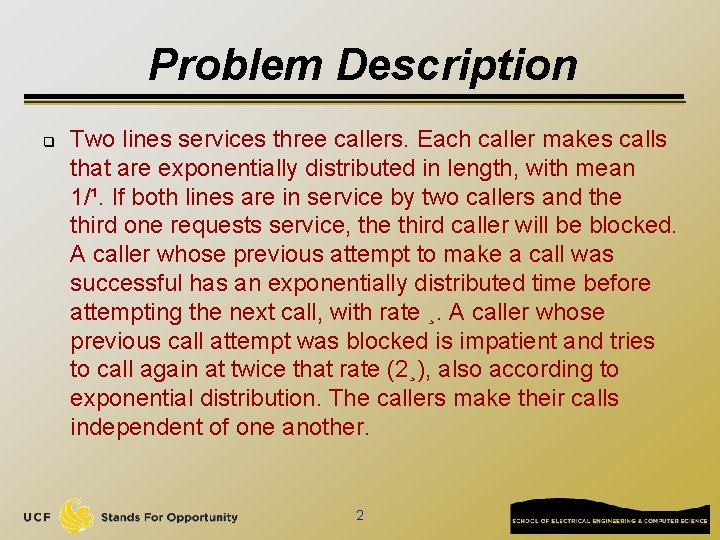
Pre Simulation q Strictly refer to the state transition diagram q q Remember current state: current. State Determine next state: next. State This is a continuous-time Markov Chain Method #1: q State duration time (for the transition node in the ¸ right): q q q Exp. distr. with rate (¸ + ¹ ) Determine the next transition event time At the time of transition event: q Use discrete r. v. simulation method to determine next. State: q Transit first path with prob. of ¸/(¸+¹) q Transit second path with prob. of ¹/(¸+¹) 5 ¹

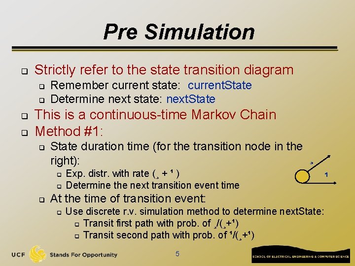
Pre Simulation q q Each node in the Markov chain has different # of outgoing jumps, how to find the combined outgoing rate? (¸ + ¹ ) in the right graph This combined rate is the diagonal entry value in Q matrix, check the three caller example: 6 ¸ ¹

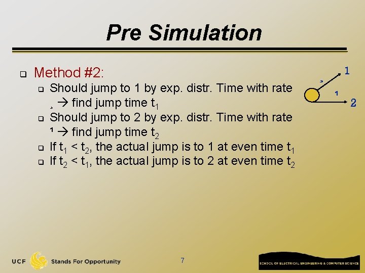
Pre Simulation q Method #2: q q Should jump to 1 by exp. distr. Time with rate ¸ find jump time t 1 Should jump to 2 by exp. distr. Time with rate ¹ find jump time t 2 If t 1 < t 2, the actual jump is to 1 at even time t 1 If t 2 < t 1, the actual jump is to 2 at even time t 2 7 1 ¸ ¹ 2

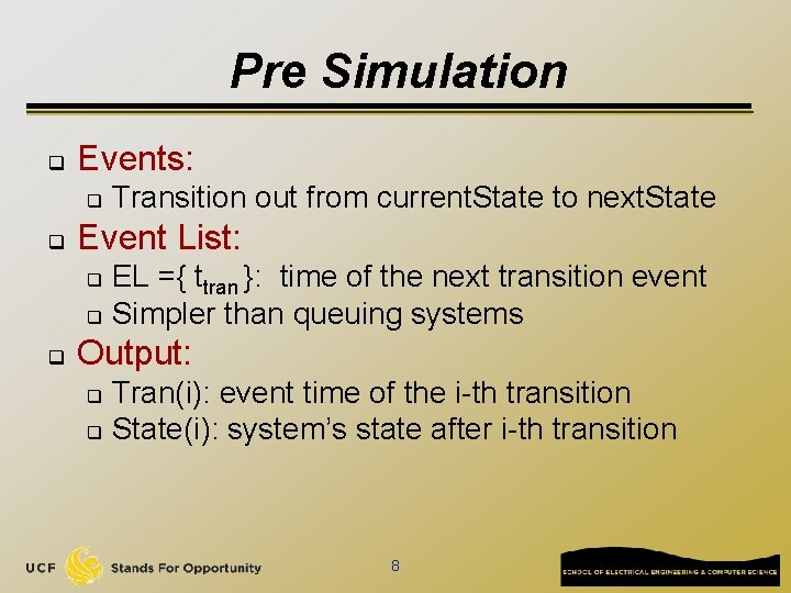
Pre Simulation q Events: q q Transition out from current. State to next. State Event List: EL ={ ttran }: time of the next transition event q Simpler than queuing systems q q Output: Tran(i): event time of the i-th transition q State(i): system’s state after i-th transition q 8

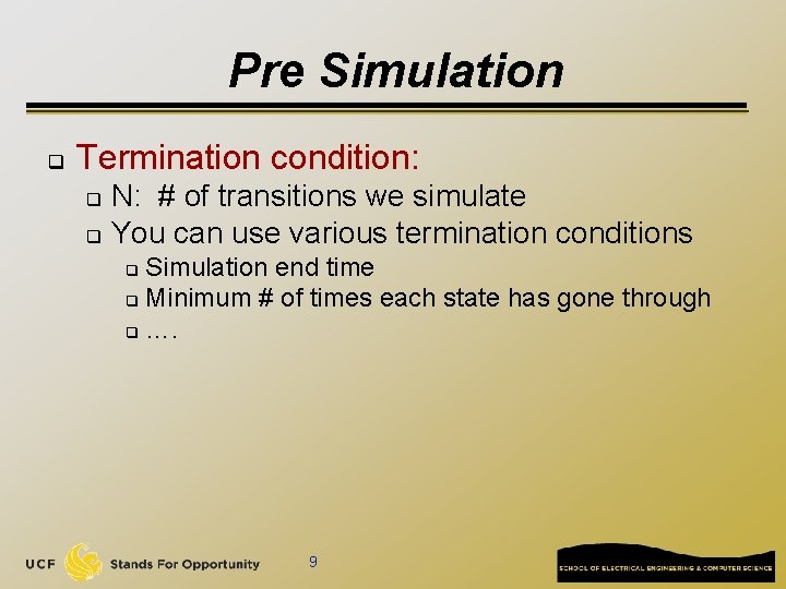
Pre Simulation q Termination condition: N: # of transitions we simulate q You can use various termination conditions q Simulation end time q Minimum # of times each state has gone through q …. q 9

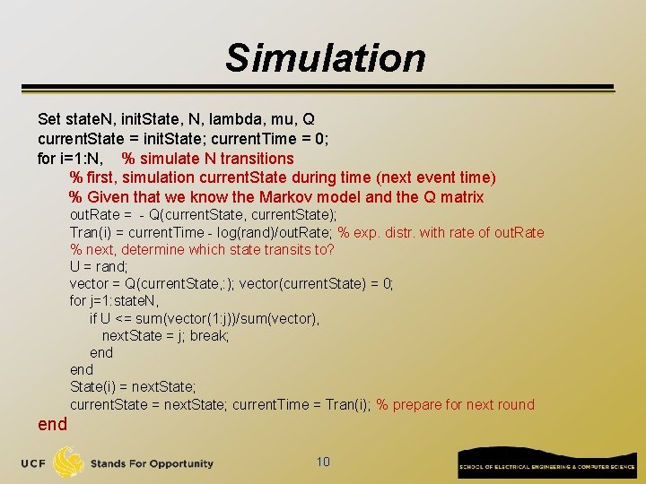
Simulation Set state. N, init. State, N, lambda, mu, Q current. State = init. State; current. Time = 0; for i=1: N, % simulate N transitions % first, simulation current. State during time (next event time) % Given that we know the Markov model and the Q matrix out. Rate = - Q(current. State, current. State); Tran(i) = current. Time - log(rand)/out. Rate; % exp. distr. with rate of out. Rate % next, determine which state transits to? U = rand; vector = Q(current. State, : ); vector(current. State) = 0; for j=1: state. N, if U <= sum(vector(1: j))/sum(vector), next. State = j; break; end State(i) = next. State; current. State = next. State; current. Time = Tran(i); % prepare for next round end 10

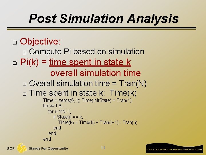
Post Simulation Analysis q Objective: q q Compute Pi based on simulation Pi(k) = time spent in state k overall simulation time Overall simulation time = Tran(N) q Time spent in state k: Time(k) q Time = zeros(6, 1); Time(init. State) = Tran(1); for k=1: 6, for i=1: N-1, if State(i) == k, Time(k) = Time(k) + Tran(i+1) - Tran(i); end end 11

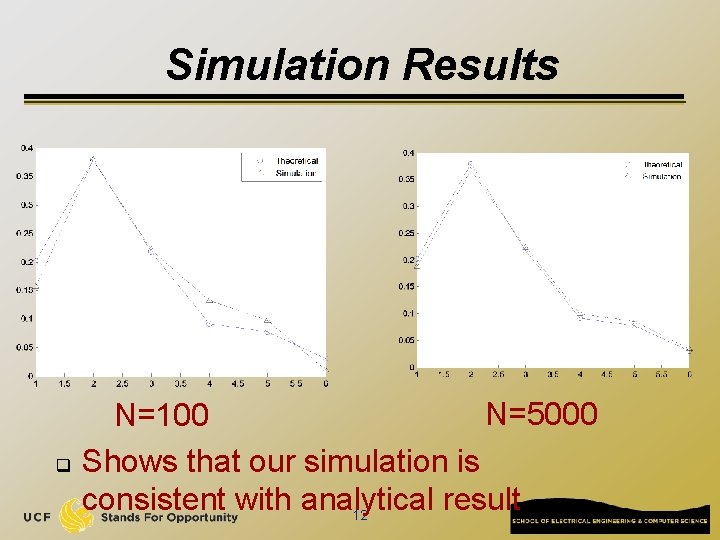
Simulation Results q N=5000 N=100 Shows that our simulation is consistent with analytical result 12

Realistic Simulation With physical meaning 13

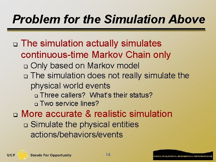
Problem for the Simulation Above q The simulation actually simulates continuous-time Markov Chain only Only based on Markov model q The simulation does not really simulate the physical world events q Three callers? What’s their status? q Two service lines? q q More accurate & realistic simulation q Simulate the physical entities actions/behaviors/events 14

Pre Simulation q What physical entities should we consider? Should directly correspond to physical entities q Should uniquely define system status q q There are two types of entities Two service lines q Three callers q q If we do not care which service line is working q We should treat three callers as simulation nodes 15

Pre Simulation q Each caller’s data: q status: ‘patient’, ‘impatient’, ‘calling’ q Caller[3]; each entry = ‘P’ or ‘I’ or ‘C’ q q In C programming, you can use ‘enum’ to define such variable next. T: event time for its next action q What “next action” could be? q Finishing phone call q q When current status is ‘calling’ Making phone call attempt q When current status is ‘idle’ or ‘impatient’ 16

Pre Simulation q Event list: q q Each caller only has one next event/action Therefore, Event list should be Event. List[3] q q Three nodes’ next action time We do not really need to save next. T in caller data since it is saved in Event. List 17

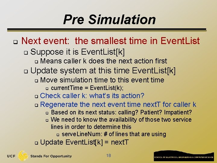
Pre Simulation q Next event: the smallest time in Event. List q Suppose it is Event. List[k] q q Means caller k does the next action first Update system at this time Event. List[k] q Move simulation time to this event time q current. Time = Event. List(k); Check caller k: what’s its action? q Regenerate the next event time next. T for caller k q q Based on its next status: calling? Patient? Impatient? We need to know the availability of those two service lines in order to determine this q serve. Line. Num: # of lines that are using Update Event. List[k] = next. T 18

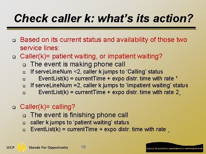
Check caller k: what’s its action? q q Based on its current status and availability of those two service lines: Caller(k)= patient waiting, or impatient waiting? q The event is making phone call q q q If serve. Line. Num <2, caller k jumps to ‘Calling’ status Event. List(k) = current. Time + expo distr. time with rate ¹ If serve. Line. Num =2, caller k jumps to ‘impatient waiting’ status Event. List(k) = current. Time + expo distr. time with rate 2¸ Caller(k)= calling? q The event is finishing phone call q q caller k jumps to ‘patient waiting’ status Event. List(k) = current. Time + expo distr. time with rate ¸ 19

Pre Simulation q Update output data: Tran(i) = Event. List[k] q State(i): system’s state after this node action q q q In order to compare with analytical results If we care about each caller’s behavior: Tran(i) = Event. List[k] q Act. Caller(i) = k q q q The k-th caller acts at time Tran(i) Caller. State(i) = Caller(k) q q k-th caller’s state after the i-th event The other callers do not change their state after this event 20

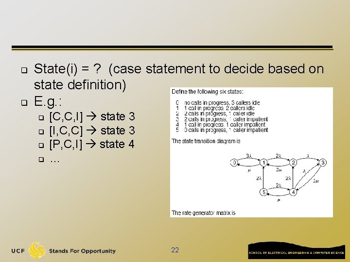
Simulation Pseudo Code Initialize N, lambda, mu, State[], Tran[] Initialize init. State and Caller[3]; current. Time = 0; Initialize Event. List[] (use corresponding distribution to generate) For i=1: N, Find the smallest time tick in Eventlist[] index is k % caller k’s action is the event we simulate now current. Time = Event. List[k]; Update caller k’s status; Update how many phone lines are used Generate caller k’s next action time, assign to Event. List[k] % Update output data Tran(i) = current. Time; State(i) = ? (case statement to decide based on state definition) End 21

q q State(i) = ? (case statement to decide based on state definition) E. g. : q q [C, C, I] state 3 [I, C, C] state 3 [P, C, I] state 4 … 22

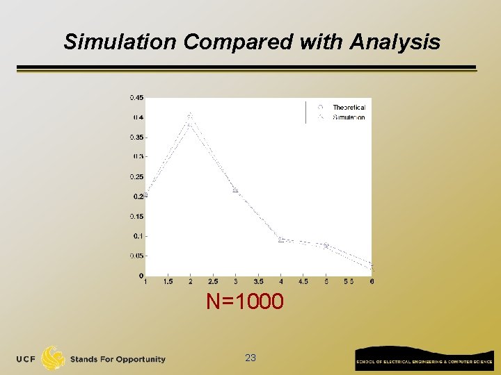
Simulation Compared with Analysis N=1000 23

Conclusion q q q The realistic simulation uses minimal amount of knowledge of statistical analysis Realistic simulation directly simulate real world entities actions and behaviors The model-based simulation is still useful q q q Better than no simulation Applicable for all systems described by one model Can study system’s performance when there is no analytical results Sometime realistic simulation is too complicated or take too long to do We need to decide which simulation to conduct 24