CDA 4150 Lecture 4 Vector Processing CRAY like

CDA 4150 Lecture 4 Vector Processing CRAY like machines

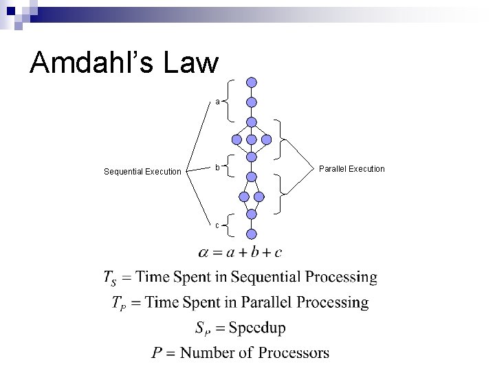
Amdahl’s Law a Sequential Execution b c Parallel Execution

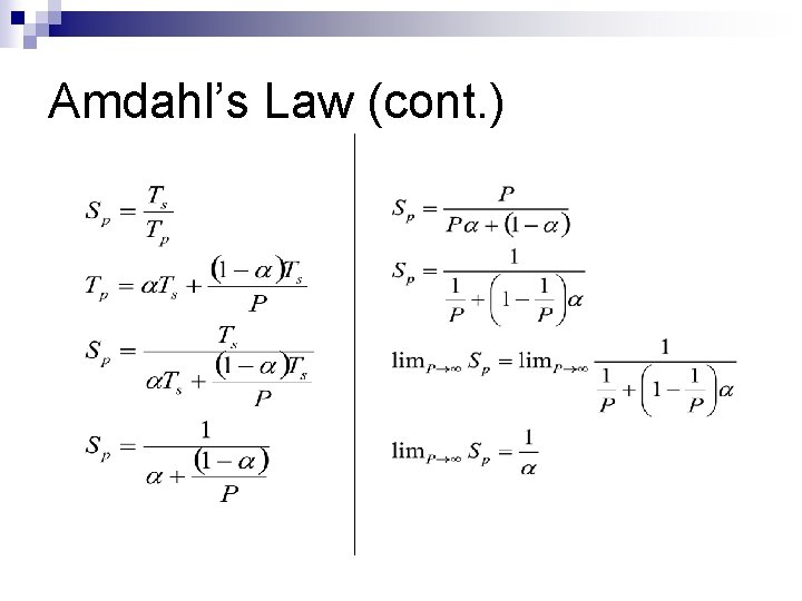
Amdahl’s Law (cont. )

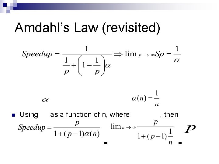
Amdahl’s Law (revisited) n Using as a function of n, where = , then =

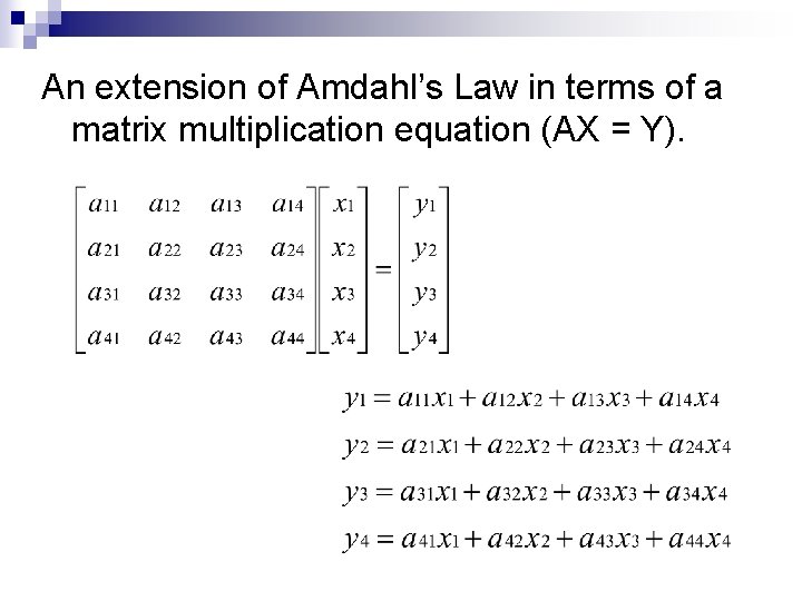
An extension of Amdahl’s Law in terms of a matrix multiplication equation (AX = Y).

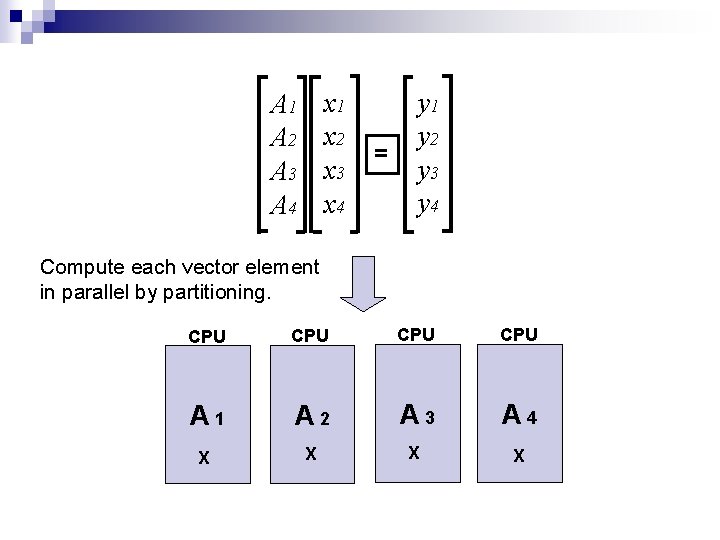
x 1 x 2 x 3 x 4 A 1 A 2 A 3 A 4 = y 1 y 2 y 3 y 4 Compute each vector element in parallel by partitioning. CPU CPU A 1 A 2 A 3 A 4 X X

R. M. Russell, “The CRAY-1 Computer System”, CACM, vol. 21, pp. 63 -72, 1978. n Introduces CRAY-1 as a vector processing Architecture

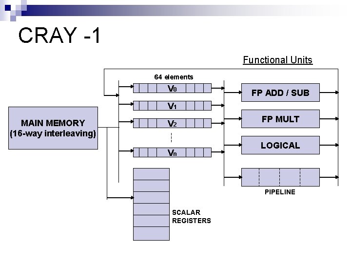
CRAY -1 Functional Units 64 elements V 0 FP ADD / SUB V 1 MAIN MEMORY (16 -way interleaving) V 2 Vn FP MULT LOGICAL PIPELINE SCALAR REGISTERS

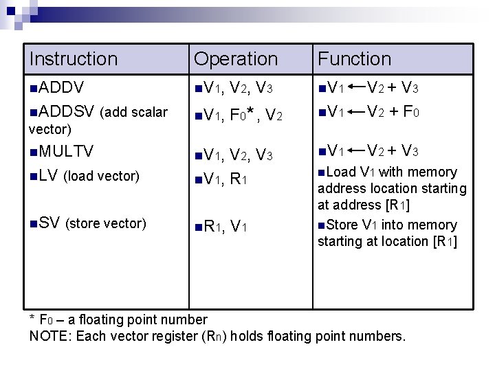
Instruction Operation Function n. ADDV n V 1, V 2, V 3 n. V 1 n. ADDSV (add scalar n V 1, F 0* , V 2 n. V 1 V 2 + V 3 V 2 + F 0 n. V 1 V 2 + V 3 vector) n. MULTV n V 1, n. LV (load vector) V 2, V 3 n V 1, R 1 n. SV (store vector) n R 1, V 1 n. Load V 1 with memory address location starting at address [R 1] n. Store V 1 into memory starting at location [R 1] * F 0 – a floating point number NOTE: Each vector register (Rn) holds floating point numbers.

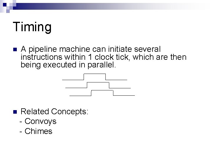
Timing n A pipeline machine can initiate several instructions within 1 clock tick, which are then being executed in parallel. n Related Concepts: - Convoys - Chimes

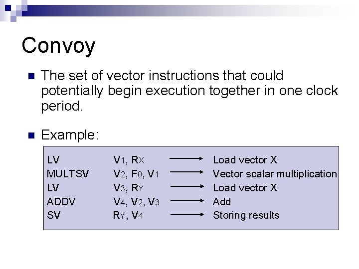
Convoy n The set of vector instructions that could potentially begin execution together in one clock period. n Example: LV MULTSV LV ADDV SV V 1, R X V 2, F 0, V 1 V 3, R Y V 4, V 2, V 3 R Y, V 4 Load vector X Vector scalar multiplication Load vector X Add Storing results

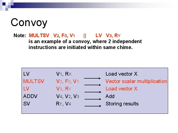
Convoy Note: MULTSV V 2, F 0, V 1 || LV V 3, RY is an example of a convoy, where 2 independent instructions are initiated within same chime. LV MULTSV LV ADDV SV V 1, R X V 2, F 0, V 1 V 3, R Y V 4, V 2, V 3 R Y, V 4 Load vector X Vector scalar multiplication Load vector X Add Storing results

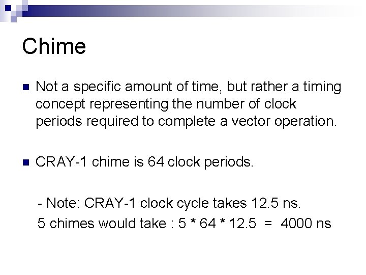
Chime n Not a specific amount of time, but rather a timing concept representing the number of clock periods required to complete a vector operation. n CRAY-1 chime is 64 clock periods. - Note: CRAY-1 clock cycle takes 12. 5 ns. 5 chimes would take : 5 * 64 * 12. 5 = 4000 ns

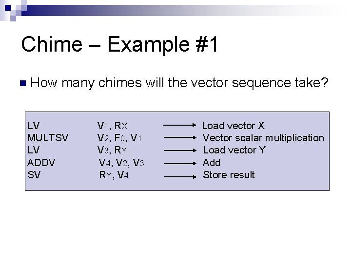
Chime – Example #1 n How many chimes will the vector sequence take? LV MULTSV LV ADDV SV V 1, R X V 2, F 0, V 1 V 3, R Y V 4, V 2, V 3 R Y, V 4 Load vector X Vector scalar multiplication Load vector Y Add Store result

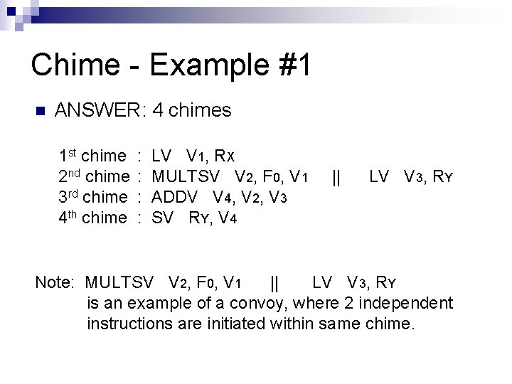
Chime - Example #1 n ANSWER: 4 chimes 1 st chime 2 nd chime 3 rd chime 4 th chime : : LV V 1, RX MULTSV V 2, F 0, V 1 ADDV V 4, V 2, V 3 SV RY, V 4 || LV V 3, RY Note: MULTSV V 2, F 0, V 1 || LV V 3, RY is an example of a convoy, where 2 independent instructions are initiated within same chime.

Chime - Example #2 n CRAY-1 For I 1 to 64 A[I] = 3. 0 * A[I] + (2. 0 + B[I]) * C[I] n To execute this: 1 st chime : V 0 2 nd chime : V 1 3 rd chime 4 th chime V 3 V 4 : V 5 V 6 V 7 : A A B 2. 0 + V 1 3. 0 * V 0 C V 3 * V 5 V 4 + V 6 V 7 Can initiate operations to use array values immediately after they have been loaded into vector registers.

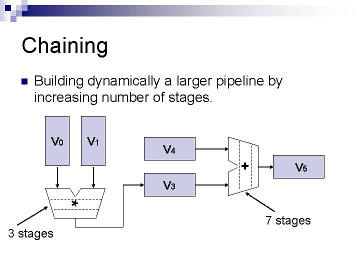
Chaining n Building dynamically a larger pipeline by increasing number of stages. V 0 V 1 V 4 + V 5 V 3 * 3 stages 7 stages

Chaining – Example #1 n For J C[J] D[J] END 1 A 1 to 64 A[J] + B[J] F[J] * E[J] are independent!! C 64 V 0 V 1 1 E + B * No chaining - these V 2 V 4 F D 64 V 3 * V 5

Chaining – Example #2 n For J C[J] D[J] END 1 to 64 A[J] * B[J] C[J] * E[J] C V 2 1 A B 64 V 0 V 1 * + V 3 E V 0 D

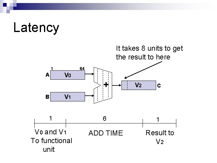
Latency It takes 8 units to get the result to here 1 A 64 V 0 + B V 2 C V 1 1 6 V 0 and V 1 To functional unit ADD TIME 1 Result to V 2

More Chaining and Storing Matrices Thanks to Dusty Price

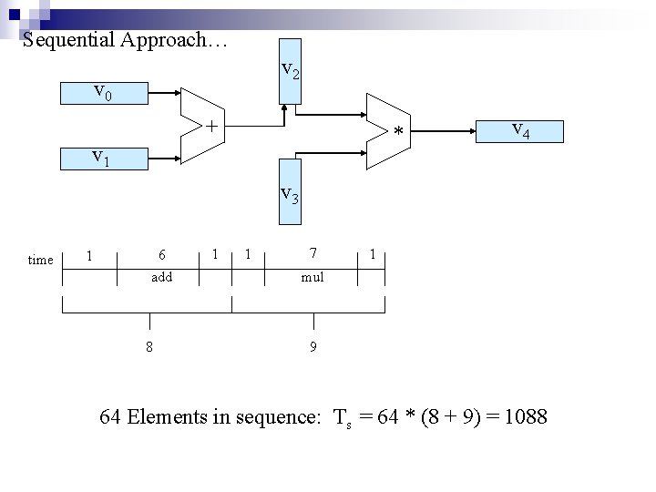
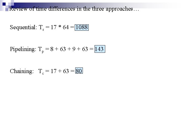
Sequential Approach… v 2 v 0 + * v 1 v 4 v 3 time 1 6 add 8 1 1 7 1 mul 9 64 Elements in sequence: Ts = 64 * (8 + 9) = 1088

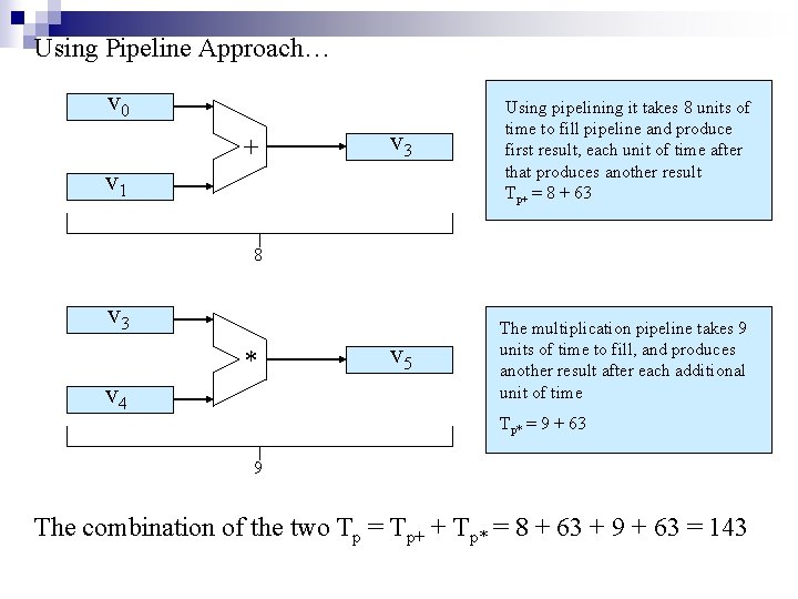
Using Pipeline Approach… v 0 + v 3 Using pipelining it takes 8 units of time to fill pipeline and produce first result, each unit of time after that produces another result Tp+ = 8 + 63 v 5 The multiplication pipeline takes 9 units of time to fill, and produces another result after each additional unit of time v 1 8 v 3 * v 4 Tp* = 9 + 63 9 The combination of the two Tp = Tp+ + Tp* = 8 + 63 + 9 + 63 = 143

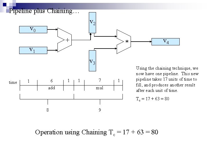
Pipeline plus Chaining… v 2 v 0 + v 1 v 3 time 1 6 add 1 v 4 * 1 7 mul 1 Using the chaining technique, we now have one pipeline. This new pipeline takes 17 units of time to fill, and produces another result after each unit of time. Tc = 17 + 63 = 80 8 9 Operation using Chaining Tc = 17 + 63 = 80

Review of time differences in the three approaches… Sequential: Ts = 17 * 64 = 1088 Pipelining: Tp = 8 + 63 + 9 + 63 = 143 Chaining: Tc = 17 + 63 = 80

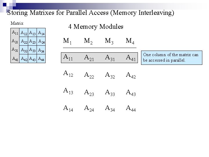
Storing Matrixes for Parallel Access (Memory Interleaving) Matrix A 11 A 12 A 13 A 14 A 21 A 22 A 23 A 24 A 31 A 32 A 33 A 34 A 41 A 42 A 43 A 44 4 Memory Modules M 1 M 2 M 3 M 4 A 11 A 21 A 31 A 41 A 12 A 22 A 32 A 42 A 13 A 23 A 33 A 43 A 14 A 24 A 34 A 44 One column of the matrix can be accessed in parallel.

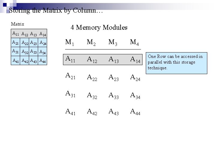
Storing the Matrix by Column… Matrix A 11 A 12 A 13 A 14 A 21 A 22 A 23 A 24 A 31 A 32 A 33 A 34 A 41 A 42 A 43 A 44 4 Memory Modules M 1 M 2 M 3 M 4 A 11 A 12 A 13 A 14 A 21 A 22 A 23 A 24 A 31 A 32 A 33 A 34 A 41 A 42 A 43 A 44 One Row can be accessed in parallel with this storage technique.

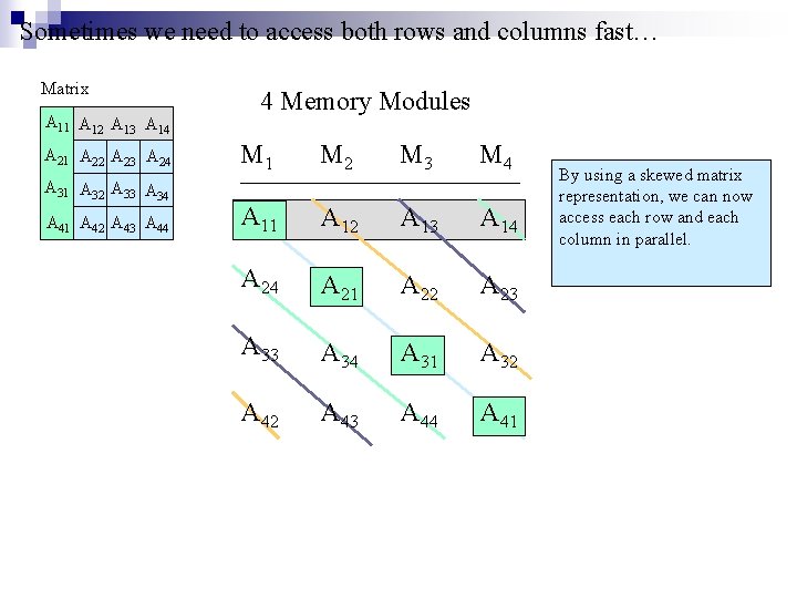
Sometimes we need to access both rows and columns fast… Matrix A 11 A 12 A 13 A 14 A 21 A 22 A 23 A 24 A 31 A 32 A 33 A 34 A 41 A 42 A 43 A 44 4 Memory Modules M 1 M 2 M 3 M 4 A 11 A 12 A 13 A 14 A 21 A 22 A 23 A 34 A 31 A 32 A 43 A 44 A 41 By using a skewed matrix representation, we can now access each row and each column in parallel.

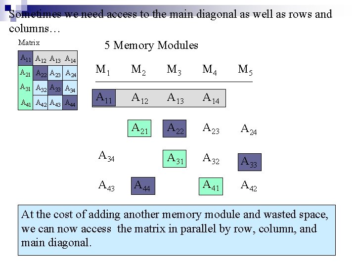
Sometimes we need access to the main diagonal as well as rows and columns… Matrix 5 Memory Modules A 11 A 12 A 13 A 14 A 21 A 22 A 23 A 24 A 31 A 32 A 33 A 34 A 41 A 42 A 43 A 44 M 1 M 2 M 3 M 4 A 11 A 12 A 13 A 14 A 21 A 22 A 23 A 24 A 31 A 32 A 33 A 41 A 42 A 34 A 43 A 44 M 5 At the cost of adding another memory module and wasted space, we can now access the matrix in parallel by row, column, and main diagonal.

Program Transformation data dependency FOR I 1 TO n do X A[I] + B[I]. . Y[I] 2 * X. . X C[I] / D[I]. . P X+2 ENDFOR removes data dependency FOR I 1 TO n do X A[I] + B[I]. . Y[I] 2 * X. . XX C[I] / D[I]. . P XX + 2 ENDFOR

Scalar Expansion FOR I 1 TO n do X A[I] + B[I]. . Y[I] 2 * X. . ENDFOR data dependency FOR I 1 TO n do X A[I] + B[I]. . Y[I] 2 * X[I]. . ENDFOR removes data dependency

Loop Unrolling FOR I 1 TO n do X[I] A[I] * B[I] ENDFOR X[1] A[1] * B[1] X[2] A[2] * B[2]. . X[n] A[n] * B[n]

Loop Fusion or Jamming FOR I 1 TO n do X[I] Y[I] * Z[I] ENDFOR I 1 TO n do M[I] P[I] + X[I] ENDFOR a) FOR I 1 TO n do X[I] Y[I] * Z[I] M[I] P[I] + X[I] ENDFOR b) FOR I 1 TO n do M[I] P[I] + Y[I] * Z[I] ENDFOR