ASCA analysis of multivariate data from an experimental

ASCA: analysis of multivariate data from an experimental design, Biosystems Data Analysis group Universiteit van Amsterdam

Contents • • ANOVA SCA ASCA Conclusions

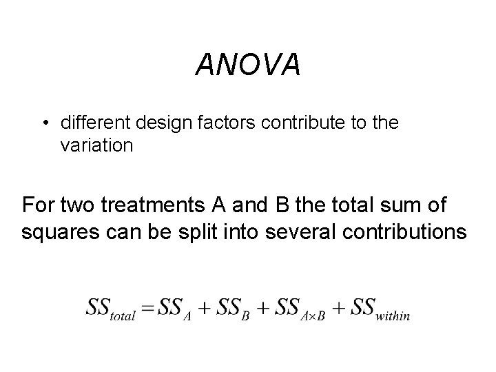
ANOVA • different design factors contribute to the variation For two treatments A and B the total sum of squares can be split into several contributions

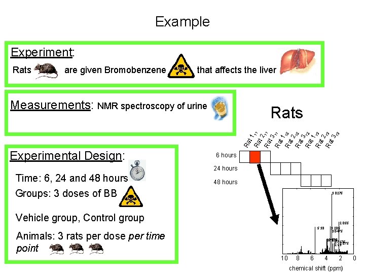
Example Experiment: Rats are given Bromobenzene that affects the liver Measurements: NMR spectroscopy of urine Ra 3 t 1 Ra 11 t 2 Ra 11 t 3 Ra 11 t 1 Ra 12 t 2 Ra 12 t 3 Ra 12 t 1 Ra 13 t 2 Ra 13 t 3 1 Rats Experimental Design: 6 hours 24 hours Time: 6, 24 and 48 hours Groups: 3 doses of BB 3. 0275 Vehicle group, Control group 2. 055 3. 285 3. 0475 5. 38 Animals: 3 rats per dose per time point 3. 675 3. 7525 2. 7175 2. 075 2. 93 10 8 6 4 2 chemical shift (ppm) 0

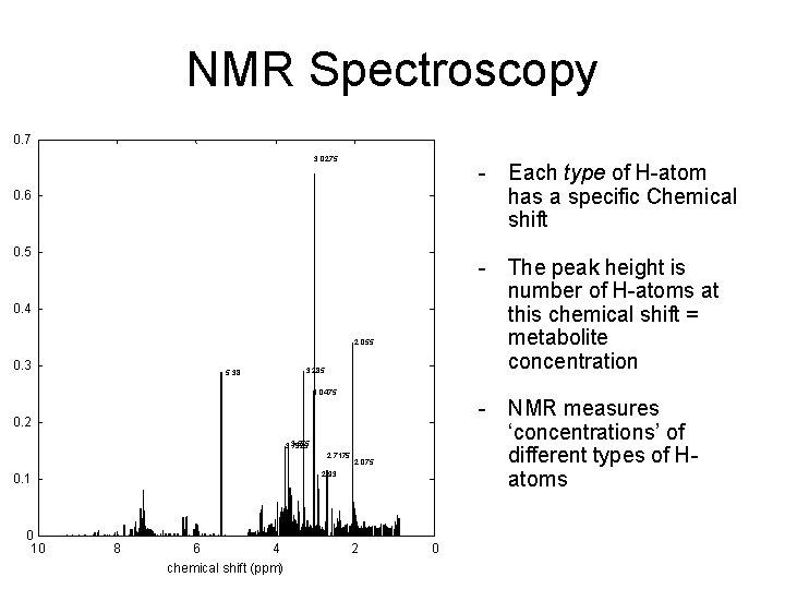
NMR Spectroscopy 0. 7 3. 0275 - Each type of H-atom has a specific Chemical shift 0. 6 0. 5 - The peak height is number of H-atoms at this chemical shift = metabolite concentration 0. 4 2. 055 0. 3 3. 285 5. 38 3. 0475 - NMR measures ‘concentrations’ of different types of Hatoms 0. 2 3. 675 3. 7525 2. 7175 0. 1 0 10 2. 075 2. 93 8 6 4 chemical shift (ppm) 2 0

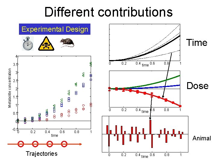
Different contributions Experimental Design Time 4 0 Metabolite concentration 3. 5 0. 2 0. 4 time 0. 6 0. 8 1 3 2. 5 Dose 2 1. 5 1 0 0. 5 0. 2 0. 4 time 0. 6 0. 8 1 0 -0. 5 0 0. 2 0. 4 time Trajectories 0. 6 0. 8 1 Animal 0 0. 2 0. 4 time 0. 6 0. 8 1

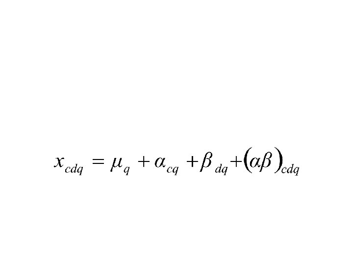
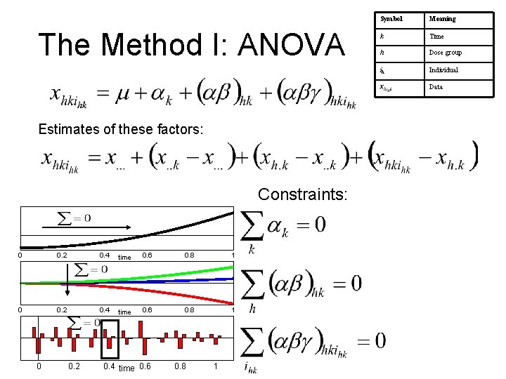
The Method I: ANOVA Symbol Meaning k Time h Dose group ih Individual Data Estimates of these factors: Constraints: 0 0. 2 0. 4 time 0. 6 0. 8 1

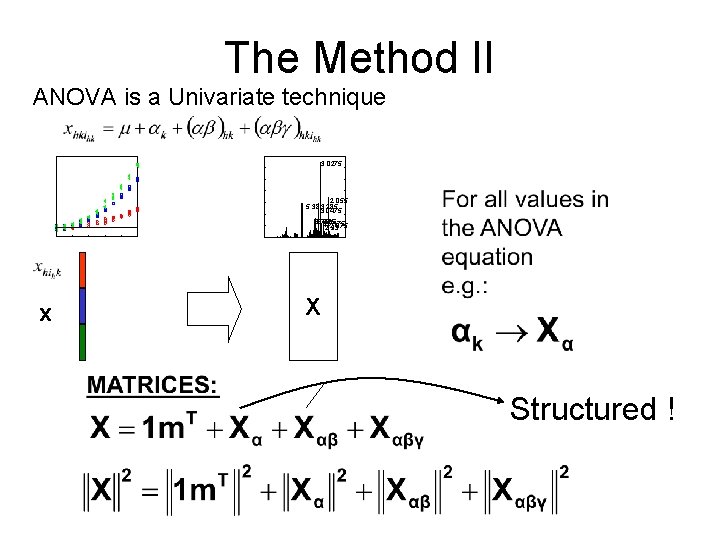
The Method II ANOVA is a Univariate technique 3. 0275 2. 055 5. 38 3. 285 3. 0475 3. 675 3. 7525 2. 7175 2. 075 2. 93 x X Structured !

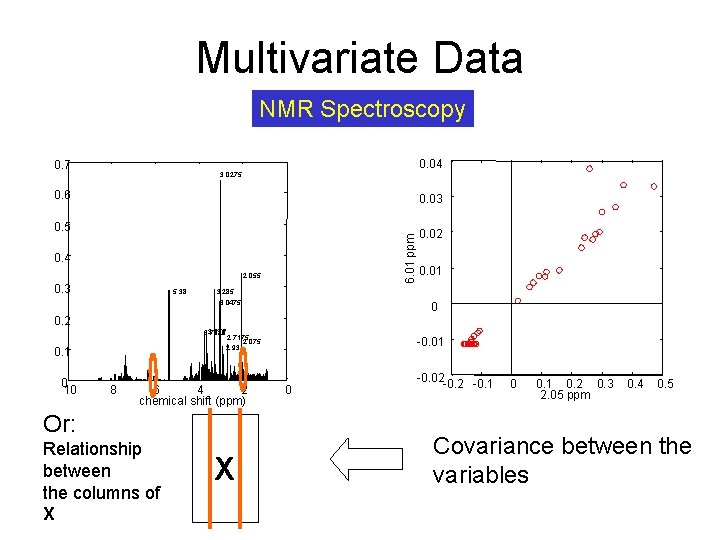
Multivariate Data NMR Spectroscopy 0. 04 0. 7 3. 0275 0. 6 0. 03 6. 01 ppm 0. 5 0. 4 2. 055 0. 3 5. 38 0. 02 0. 01 3. 285 3. 0475 0 0. 2 3. 675 3. 7525 2. 7175 2. 075 2. 93 0. 1 0 10 8 6 4 2 chemical shift (ppm) Or: Relationship between the columns of X X -0. 01 0 -0. 02 -0. 1 0. 2 0. 3 2. 05 ppm 0. 4 0. 5 Covariance between the variables

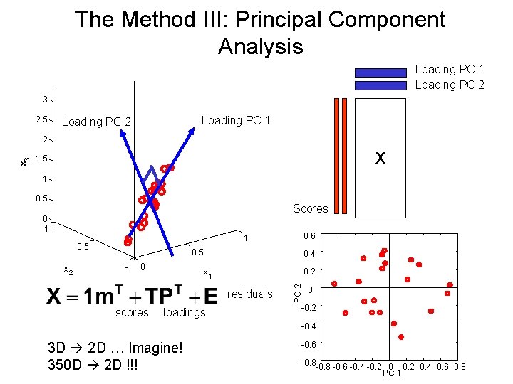
The Method III: Principal Component Analysis Loading PC 1 Loading PC 2 3 2. 5 Loading PC 1 Loading PC 2 X 1. 5 1 0. 5 Scores 0 1 0. 5 x 2 0. 6 1 0. 5 0 0 0. 4 0. 2 x 1 residuals scores loadings PC 2 x 3 2 0 -0. 2 -0. 4 3 D 2 D … Imagine! 350 D 2 D !!! -0. 6 -0. 8 -0. 6 -0. 4 -0. 2 0. 4 0. 6 0. 8 PC 1

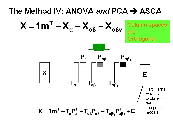
The Method IV: ANOVA and PCA ASCA Column spaces are Orthogonal E Parts of the data not explained by the component models

In Words: • ASCA models the different contributions to the variation in the data • ASCA takes the covariance between the variables into account • ASCA gives a solution for the problem at hand.

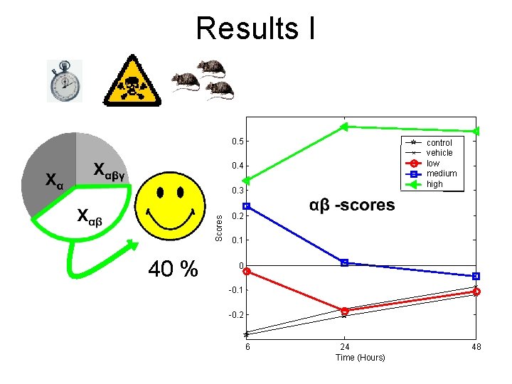
Results I 0. 5 control vehicle low medium high 0. 4 Scores 0. 3 40 % 0. 2 0. 1 0 -0. 1 -0. 2 6 24 Time (Hours) 48

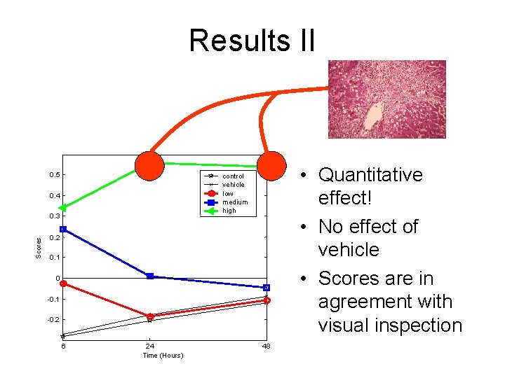
Results II 0. 5 0. 4 0. 3 Scores • Quantitative effect! • No effect of vehicle • Scores are in agreement with visual inspection control vehicle low medium high 0. 2 0. 1 0 -0. 1 -0. 2 6 24 Time (Hours) 48

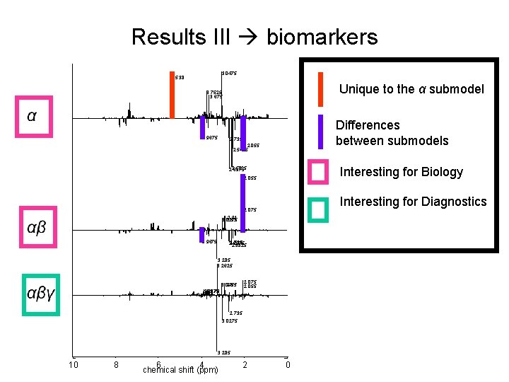
Results III biomarkers 3. 0475 5. 38 Unique to the α submodel 3. 7525 3. 675 3. 9675 Differences between submodels 2. 735 2. 055 2. 5425 Interesting for Biology 2. 5825 2. 6975 2. 055 Interesting for Diagnostics 2. 075 2. 91 3. 0275 2. 93 3. 9675 2. 735 2. 6975 2. 5825 3. 285 3. 2625 2. 93 3. 0475 3. 73 3. 8875 2. 075 2. 055 2. 735 3. 0275 3. 285 10 8 6 4 chemical shift (ppm) 2 0

Conclusions • Metabolomics (and other –omics) techniques give multivariate datasets with an underlying experimental design • For this type of data, ASCA can be used • The results observed for this experiment are in accordance with clinical observations • The metabolites that are responsible for this variation can be found using ASCA BIOMARKERS

Discussion 1. How can I perform statistics on the ASCA model? (e. g. Significance testing) 2. Are there other constraints possible for this model? (e. g. stochastic independence) 3. Are there alternative methods for solving this problem?