Multivariate Data Descriptive techniques for Multivariate data In


 for each case")

")


 • Stronger positive relationship between X and Y •")


 • Pearson’s correlation coefficient (r) • Spearman’s")


 related to either Verbal IQ or Math")


")
 Spearman’s rank correlation coefficient is computed as follows:")


 4. The value of")


 r 3 (x 1, y 1) r 1 r")


 in")


X")


 = (variability in Y explained by")


 in n =")


X")


- Slides: 169
Multivariate Data
Descriptive techniques for Multivariate data In most research situations data is collected on more than one variable (usually many variables)
Graphical Techniques • The scatter plot • The two dimensional Histogram
The Scatter Plot For two variables X and Y we will have a measurements for each variable on each case: xi, yi xi = the value of X for case i and yi = the value of Y for case i.
To Construct a scatter plot we plot the points: (xi, yi) for each case on the X-Y plane. (xi, yi) yi xi
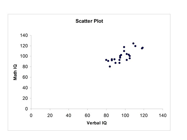
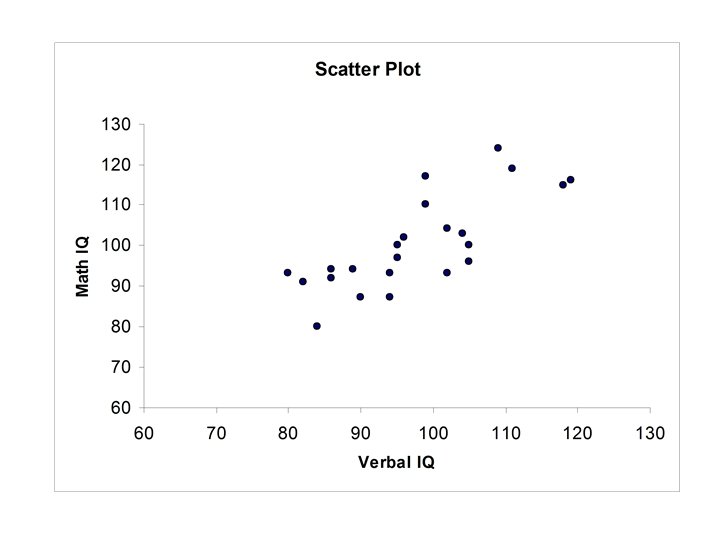
Student Verbal IQ 1 2 3 4 5 6 7 8 9 10 11 12 13 14 15 16 17 18 19 20 21 22 23 86 104 86 105 118 96 90 95 105 84 94 119 82 80 109 111 89 99 94 99 95 102 Data Set #3 The following table gives data on Verbal IQ, Math IQ, Initial Reading Acheivement Score, and Final Reading Acheivement Score for 23 students who have recently completed a reading improvement program Initial Final Math Reading IQ Acheivement 94 103 92 100 115 102 87 100 96 80 87 116 91 93 124 119 94 117 93 110 97 104 93 1. 1 1. 5 2. 0 1. 9 1. 4 1. 5 1. 4 1. 7 1. 6 1. 7 1. 2 1. 0 1. 8 1. 4 1. 6 1. 4 1. 5 1. 7 1. 6 1. 7 1. 9 2. 0 3. 5 2. 4 1. 8 2. 0 1. 7 3. 1 1. 8 1. 7 2. 5 3. 0 1. 8 2. 6 1. 4 2. 0 1. 3 3. 1 1. 9
(84, 80)
Some Scatter Patterns
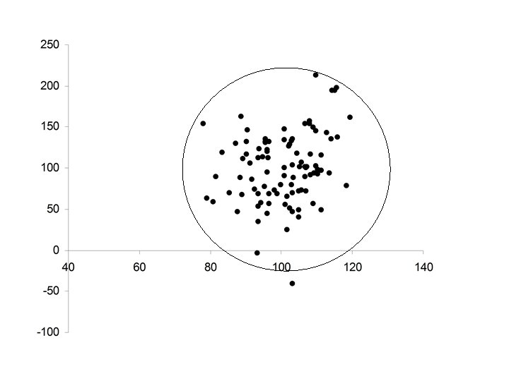
• Circular • No relationship between X and Y • Unable to predict Y from X
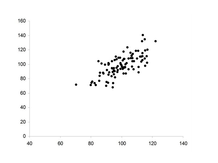
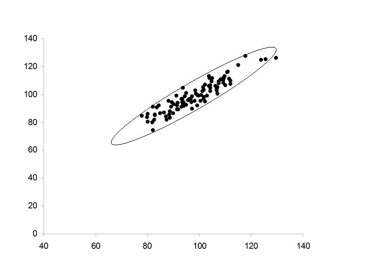
• Ellipsoidal • Positive relationship between X and Y • Increases in X correspond to increases in Y (but not always) • Major axis of the ellipse has positive slope
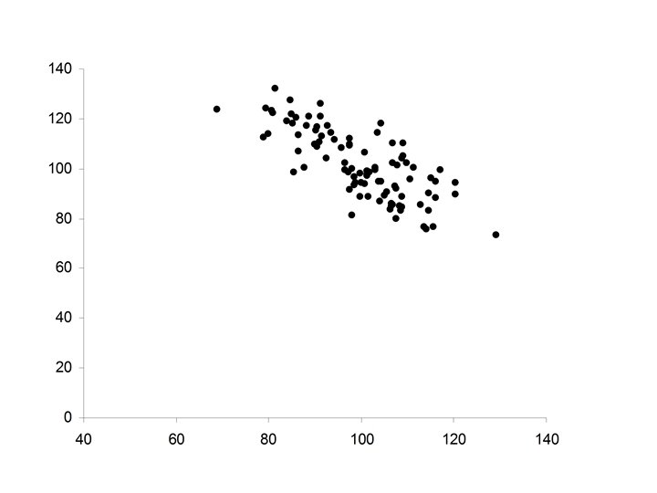
Example Verbal IQ, Math. IQ
Some More Patterns
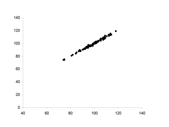
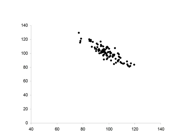
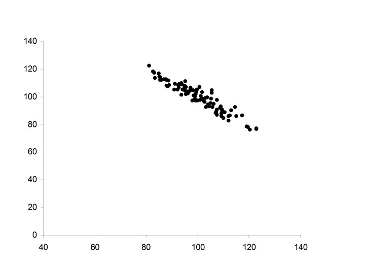
• Ellipsoidal (thinner ellipse) • Stronger positive relationship between X and Y • Increases in X correspond to increases in Y (more freqequently) • Major axis of the ellipse has positive slope • Minor axis of the ellipse much smaller
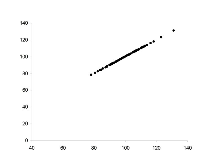
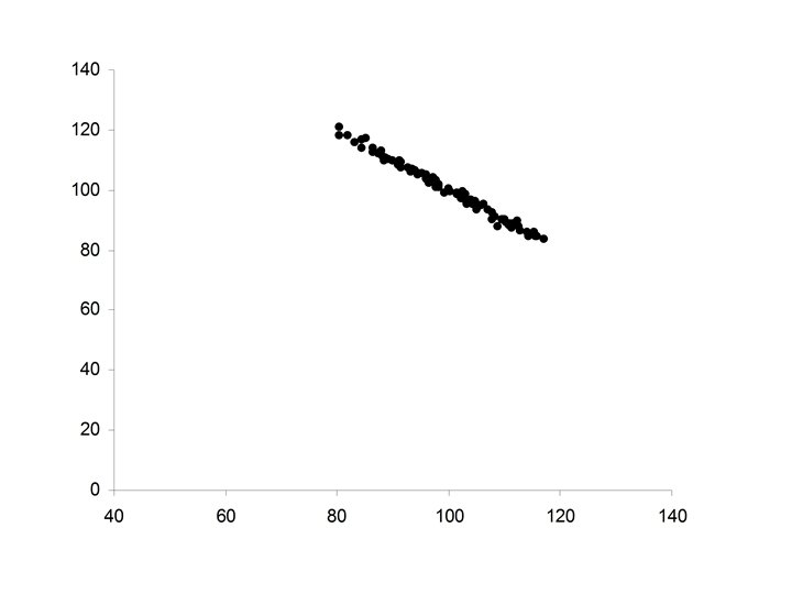
• Increased strength in the positive relationship between X and Y • Increases in X correspond to increases in Y (almost always) • Minor axis of the ellipse extremely small in relationship to the Major axis of the ellipse.
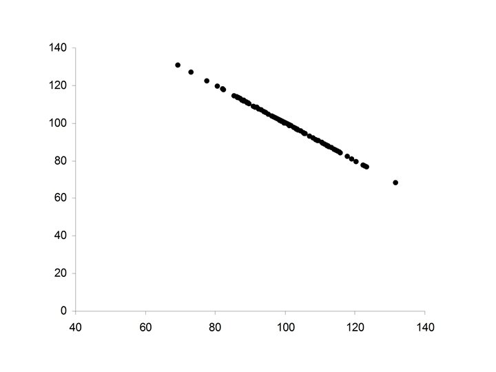
• Perfect positive relationship between X and Y • Y perfectly predictable from X • Data falls exactly along a straight line with positive slope
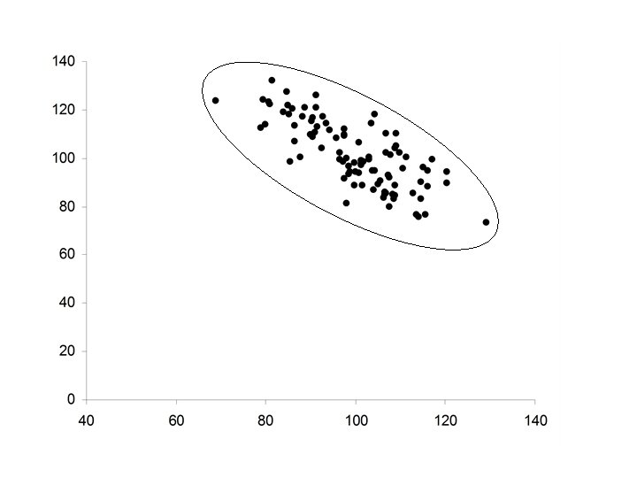
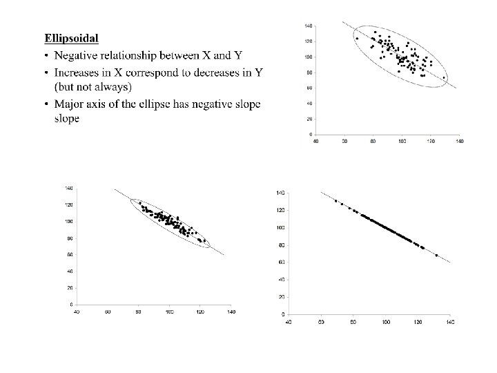
• Ellipsoidal • Negative relationship between X and Y • Increases in X correspond to decreases in Y (but not always) • Major axis of the ellipse has negative slope
• The strength of the relationship can increase until changes in Y can be perfectly predicted from X
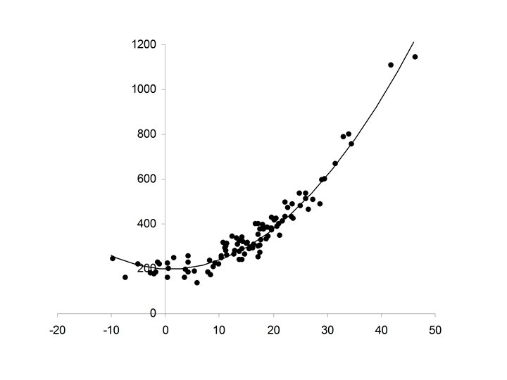
Some Non-Linear Patterns
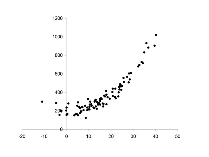
• In a Linear pattern Y increase with respect to X at a constant rate • In a Non-linear pattern the rate that Y increases with respect to X is variable
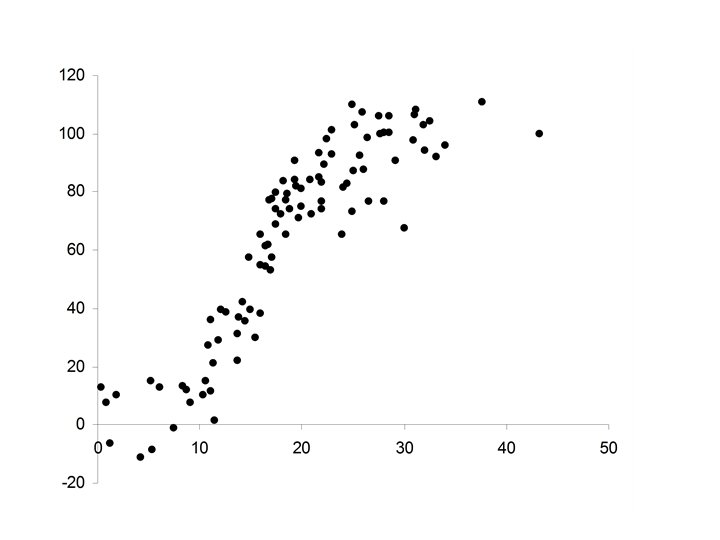
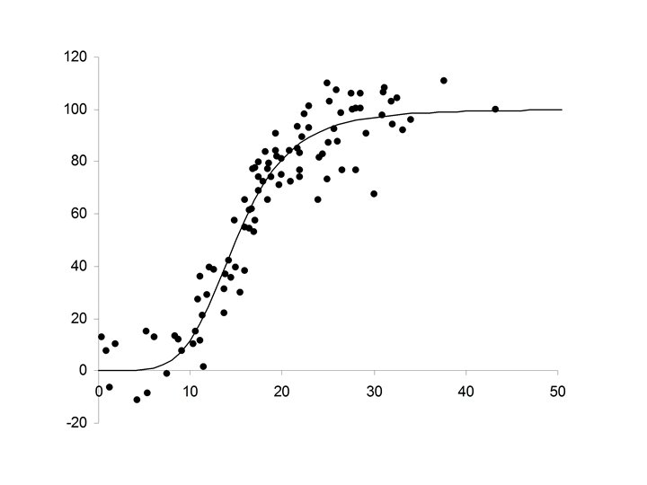
Growth Patterns
• Growth patterns frequently follow a sigmoid curve • Growth at the start is slow • It then speeds up • Slows down again as it reaches it limiting size
Review the scatter plot
Some Scatter Patterns
Non-Linear Patterns
Measures of strength of a relationship (Correlation) • Pearson’s correlation coefficient (r) • Spearman’s rank correlation coefficient (rho, r)
Assume that we have collected data on two variables X and Y. Let (x 1, y 1) (x 2, y 2) (x 3, y 3) … (xn, yn) denote the pairs of measurements on the on two variables X and Y for n cases in a sample (or population)
From this data we can compute summary statistics for each variable. The means and
The standard deviations and
These statistics: • give information for each variable separately but • give no information about the relationship between the two variables
Consider the statistics:
The first two statistics: and • are used to measure variability in each variable • they are used to compute the sample standard deviations
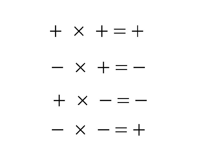
The third statistic: • is used to measure correlation • If two variables are positively related the sign of will agree with the sign of
• When is positive will be positive. • When xi is above its mean, yi will be above its mean • When is negative will be negative. • When xi is below its mean, yi will be below its mean The product will be positive for most cases.
This implies that the statistic • will be positive • Most of the terms in this sum will be positive
On the other hand • If two variables are negatively related the sign of will be opposite in sign to
• When is positive will be negative. • When xi is above its mean, yi will be below its mean • When is negative will be positive. • When xi is below its mean, yi will be above its mean The product will be negative for most cases.
Again implies that the statistic • will be negative • Most of the terms in this sum will be negative
Pearson’s correlation coefficient r A statistic measuring the strength of the relationship between two variables - X and Y
Pearsons correlation coefficient is defined as below:
The denominator: is always positive
The numerator: • is positive if there is a positive relationship between X ad Y and • negative if there is a negative relationship between X ad Y. • This property carries over to Pearson’s correlation coefficient r
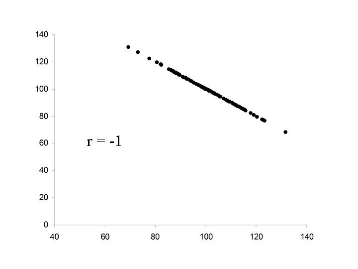
Properties of Pearson’s correlation coefficient r 1. The value of r is always between – 1 and +1. 2. If the relationship between X and Y is positive, then r will be positive. 3. If the relationship between X and Y is negative, then r will be negative. 4. If there is no relationship between X and Y, then r will be zero. 5. The value of r will be +1 if the points, (xi, yi) lie on a straight line with positive slope. 6. The value of r will be -1 if the points, (xi, yi) lie on a straight line with negative slope.
r =1
r = 0. 95
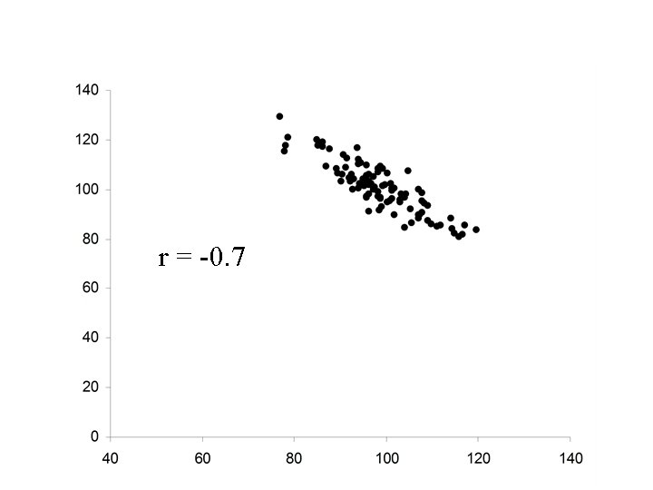
r = 0. 7
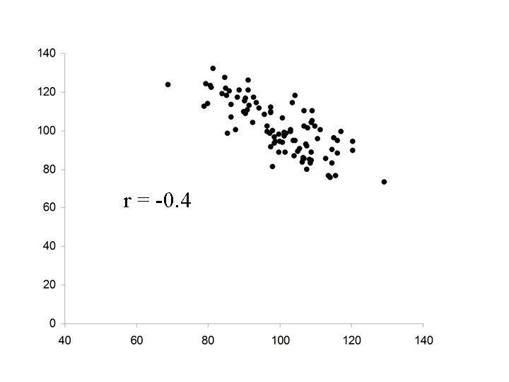
r = 0. 4
r = 0
r = -0. 95
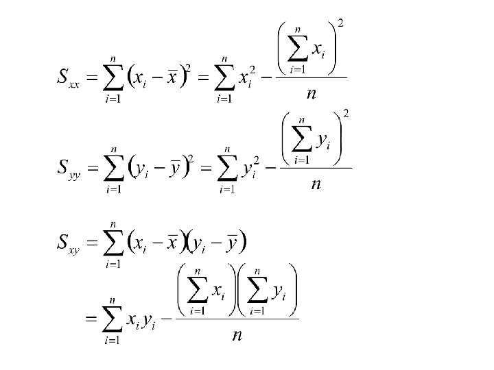
Computing formulae for the statistics:
To compute first compute Then
Example Verbal IQ, Math. IQ
Student Verbal IQ 1 2 3 4 5 6 7 8 9 10 11 12 13 14 15 16 17 18 19 20 21 22 23 86 104 86 105 118 96 90 95 105 84 94 119 82 80 109 111 89 99 94 99 95 102 Data Set #3 The following table gives data on Verbal IQ, Math IQ, Initial Reading Acheivement Score, and Final Reading Acheivement Score for 23 students who have recently completed a reading improvement program Initial Final Math Reading IQ Acheivement 94 103 92 100 115 102 87 100 96 80 87 116 91 93 124 119 94 117 93 110 97 104 93 1. 1 1. 5 2. 0 1. 9 1. 4 1. 5 1. 4 1. 7 1. 6 1. 7 1. 2 1. 0 1. 8 1. 4 1. 6 1. 4 1. 5 1. 7 1. 6 1. 7 1. 9 2. 0 3. 5 2. 4 1. 8 2. 0 1. 7 3. 1 1. 8 1. 7 2. 5 3. 0 1. 8 2. 6 1. 4 2. 0 1. 3 3. 1 1. 9
Now Hence
Thus Pearsons correlation coefficient is:
Thus r = 0. 769 • Verbal IQ and Math IQ are positively correlated. • If Verbal IQ is above (below) the mean then for most cases Math IQ will also be above (below) the mean.
Is the improvement in reading achievement (RA) related to either Verbal IQ or Math IQ? improvement in RA = Final RA – Initial RA
The Data Correlation between Math IQ and RA Improvement Correlation between Verbal IQ and RA Improvement
Scatterplot: Math IQ vs RA Improvement
Scatterplot: Verbal IQ vs RA Improvement
Spearman’s rank correlation coefficient r (rho)
Spearman’s rank correlation coefficient r (rho) Spearman’s rank correlation coefficient is computed as follows: • Arrange the observations on X in increasing order and assign them the ranks 1, 2, 3, …, n • Arrange the observations on Y in increasing order and assign them the ranks 1, 2, 3, …, n. • For any case (i) let (xi, yi) denote the observations on X and Y and let (ri, si) denote the ranks on X and Y.
• If the variables X and Y are strongly positively correlated the ranks on X should generally agree with the ranks on Y. (The largest X should be the largest Y, The smallest X should be the smallest Y). • If the variables X and Y are strongly negatively correlated the ranks on X should in the reverse order to the ranks on Y. (The largest X should be the smallest Y, The smallest X should be the largest Y). • If the variables X and Y are uncorrelated the ranks on X should randomly distributed with the ranks on Y.
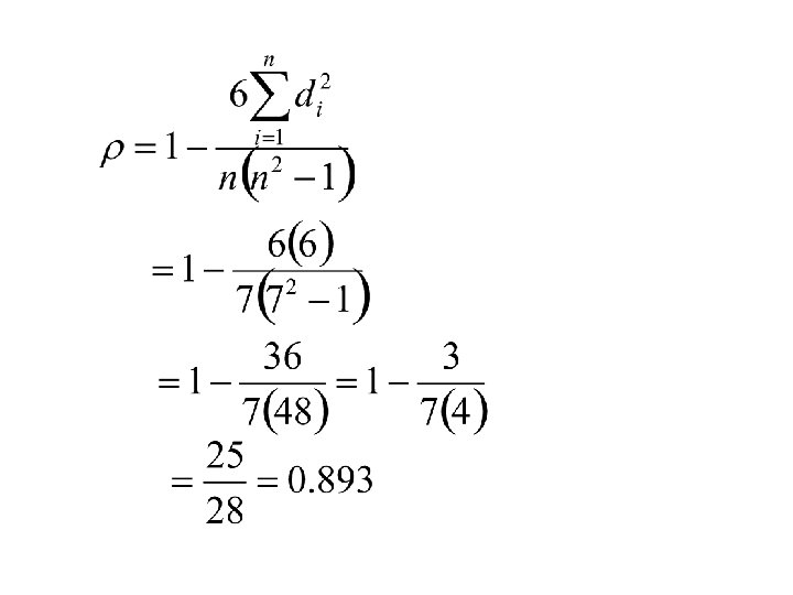
Spearman’s rank correlation coefficient is defined as follows: For each case let di = ri – si = difference in the two ranks. Then Spearman’s rank correlation coefficient (r) is defined as follows:
Properties of Spearman’s rank correlation coefficient r 1. The value of r is always between – 1 and +1. 2. If the relationship between X and Y is positive, then r will be positive. 3. If the relationship between X and Y is negative, then r will be negative. 4. If there is no relationship between X and Y, then r will be zero. 5. The value of r will be +1 if the ranks of X completely agree with the ranks of Y. 6. The value of r will be -1 if the ranks of X are in reverse order to the ranks of Y.
Example xi 25. 0 33. 9 16. 7 37. 4 24. 6 17. 3 40. 2 yi 24. 3 38. 7 13. 4 32. 1 28. 0 12. 5 44. 9 Ranking the X’s and the Y’s we get: ri 4 5 1 6 3 2 7 si 3 6 2 5 4 1 7 Computing the differences in ranks gives us: di 1 -1 -1 1 0
Computing Pearsons correlation coefficient, r, for the same problem:
To compute first compute
Then
and Compare with
Comments: Spearman’s rank correlation coefficient r and Pearson’s correlation coefficient r 1. The value of r can also be computed from: 2. Spearman’s r is Pearson’s r computed from the ranks.
3. Spearman’s r is less sensitive to extreme observations. (outliers) 4. The value of Pearson’s r is much more sensitive to extreme outliers. This is similar to the comparison between the median and the mean, the standard deviation and the pseudo-standard deviation. The mean and standard deviation are more sensitive to outliers than the median and pseudo- standard deviation.
Scatter plots
Some Scatter Patterns
Non-Linear Patterns
Measuring correlation 1. Pearson’s correlation coefficient r 2. Spearman’s rank correlation coefficient r
Simple Linear Regression Fitting straight lines to data
The Least Squares Line The Regression Line • When data is correlated it falls roughly about a straight line.
In this situation wants to: • Find the equation of the straight line through the data that yields the best fit. The equation of any straight line: is of the form: Y = a + b. X b = the slope of the line a = the intercept of the line
Rise = y 2 -y 1 Run = x 2 -x 1 a y 2 -y 1 Rise b = Run = x -x 2 1
• a is the value of Y when X is zero • b is the rate that Y increases per unit increase in X. • For a straight line this rate is constant. • For non linear curves the rate that Y increases per unit increase in X varies with X.
Linear
Non-linear
Example: In the following example both blood pressure and age were measure for each female subject. Subjects were grouped into age classes and the median Blood Pressure measurement was computed for each age class. He data are summarized below: Age Class 30 -40 40 -50 50 -60 60 -70 70 -80 Mipoint Age (X) 35 45 55 65 75 Median BP (Y) 114 124 143 158 166
Graph:
Interpretation of the slope and intercept 1. Intercept – value of Y at X = 0. – Predicted Blood pressure of a newborn (65. 1). – This interpretation remains valid only if linearity is true down to X = 0. 2. Slope – rate of increase in Y per unit increase in X. – Blood Pressure increases 1. 38 units each year.
The Least Squares Line Fitting the best straight line to “linear” data
Reasons for fitting a straight line to data 1. It provides a precise description of the relationship between Y and X. 2. The interpretation of the parameters of the line (slope and intercept) leads to an improved understanding of the phenomena that is under study. 3. The equation of the line is useful for prediction of the dependent variable (Y) from the independent variable (X).
Assume that we have collected data on two variables X and Y. Let (x 1, y 1) (x 2, y 2) (x 3, y 3) … (xn, yn) denote the pairs of measurements on the on two variables X and Y for n cases in a sample (or population)
Let Y=a +b. X denote an arbitrary equation of a straight line. a and b are known values. This equation can be used to predict for each value of X, the value of Y. For example, if X = xi (as for the ith case) then the predicted value of Y is:
For example if Y = a + b X = 25. 2 + 2. 0 X Is the equation of the straight line. and if X = xi = 20 (for the ith case) then the predicted value of Y is:
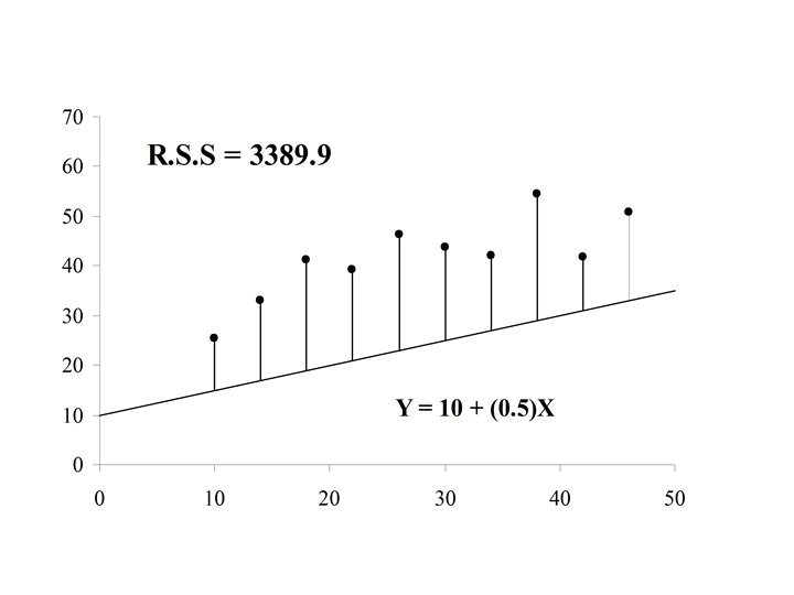
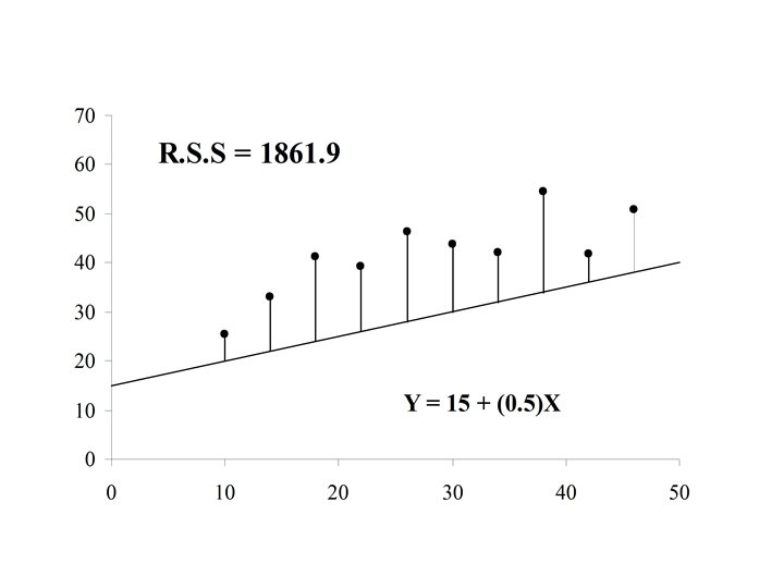
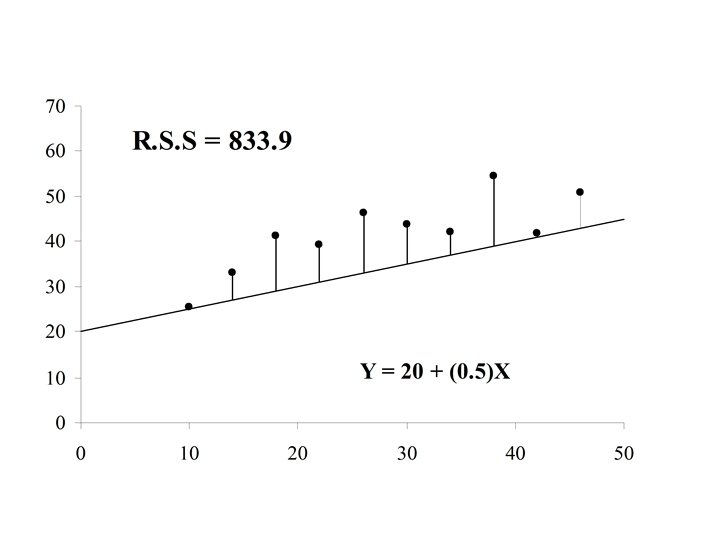
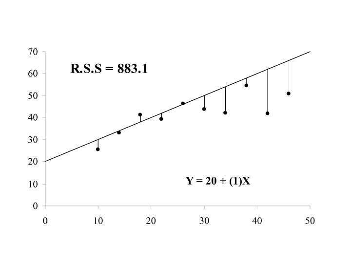
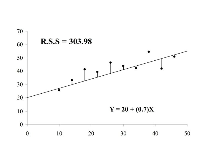
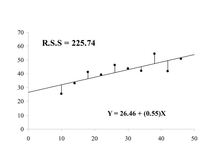
If the actual value of Y is yi = 70. 0 for case i, then the difference is the error in the prediction for case i. is also called the residual for case i
If the residual can be computed for each case in the sample, The residual sum of squares (RSS) is a measure of the “goodness of fit of the line Y = a + b. X to the data
Y (x 3, y 3) r 3 (x 1, y 1) r 1 r 4 (x 4, y 4) Y=a+b. X r 2 (x 2, y 2) X
The optimal choice of a and b will result in the residual sum of squares attaining a minimum. If this is the case than the line: Y = a + b. X is called the Least Squares Line
The equation for the least squares line Let
Computing Formulae:
Then the slope of the least squares line can be shown to be:
and the intercept of the least squares line can be shown to be:
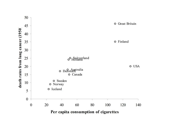
The following data showed the per capita consumption of cigarettes per month (X) in various countries in 1930, and the death rates from lung cancer for men in 1950. TABLE : Per capita consumption of cigarettes per month (Xi) in n = 11 countries in 1930, and the death rates, Yi (per 100, 000), from lung cancer for men in 1950. Country (i) Xi Yi Australia 48 18 Canada 50 15 Denmark 38 17 Finland 110 35 Great Britain 110 46 Holland 49 24 Iceland 23 6 Norway 25 9 Sweden 30 11 Switzerland 51 25 USA 130 20
Fitting the Least Squares Line
Fitting the Least Squares Line First compute the following three quantities:
Computing Estimate of Slope and Intercept
Y = 6. 756 + (0. 228)X
Interpretation of the slope and intercept 1. Intercept – value of Y at X = 0. – Predicted death rate from lung cancer (6. 756) for men in 1950 in Counties with no smoking in 1930 (X = 0). 2. Slope – rate of increase in Y per unit increase in X. – Death rate from lung cancer for men in 1950 increases 0. 228 units for each increase of 1 cigarette per capita consumption in 1930.
Correlation & Linear Regression A review
The Scattergram Pearson’s Correlation Coefficient Spearman’s Rank Correlation Coefficient
The Least squares Line Slope and intercept
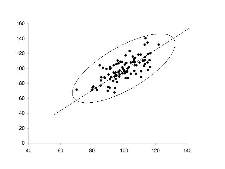
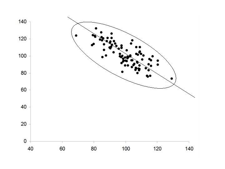
Comment: Regression to the mean The Least Squares line is not the major axis of the ellipse that covers the data. The major axis of the ellipse The Least Squares line
• If slope of the major axis is positive, the slope of the Least Squares line will also be positive but not as large • This fact is sometimes revered to as regression towards the mean • Suppose X is the father’s height and Y is the son’s height. If the fathers is tall within his population, then the son will also likely be tall but not as tall as the father within his population.
Relationship between correlation and Linear Regression 1. Pearsons correlation. • Takes values between – 1 and +1
2. Least squares Line Y = a + b. X – Minimises the Residual Sum of Squares: – The Sum of Squares that measures the variability in Y that is unexplained by X. – This can also be denoted by: SSunexplained
Some other Sum of Squares: – The Sum of Squares that measures the total variability in Y (ignoring X).
– The Sum of Squares that measures the total variability in Y that is explained by X.
It can be shown: (Total variability in Y) = (variability in Y explained by X) + (variability in Y unexplained by X)
It can also be shown: = proportion variability in Y explained by X. = the coefficient of determination
Further: = proportion variability in Y that is unexplained by X.
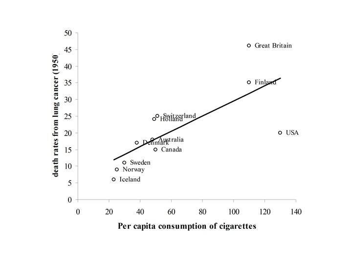
Example TABLE : Per capita consumption of cigarettes per month (Xi) in n = 11 countries in 1930, and the death rates, Yi (per 100, 000), from lung cancer for men in 1950. Country (i) Xi Yi Australia 48 18 Canada 50 15 Denmark 38 17 Finland 110 35 Great Britain 110 46 Holland 49 24 Iceland 23 6 Norway 25 9 Sweden 30 11 Switzerland 51 25 USA 130 20
Fitting the Least Squares Line First compute the following three quantities:
Computing Estimate of Slope and Intercept
Computing r and r 2 54. 4% of the variability in Y (death rate due to lung Cancer (1950) is explained by X (per capita cigarette smoking in 1930)
Y = 6. 756 + (0. 228)X
Comments • Correlation will be +1 or -1 if the data lies on a straight line. • Correlation can be zero or close to zero if the data is either – Not related or – In some situations non-linear
Example The data
One should be careful in interpreting zero correlation. It does not necessarily imply that Y is not related to X. It could happen that Y is non-linearly related to X. One should plot Y vs X before concluding that Y is not related to X.
Next topic: Categorical Data