An Efficient Data Envelopment Analysis with a large

An Efficient Data Envelopment Analysis with a large data set in Stata 15 -16 July, 2010 Boston 10 Stata Conference Choonjoo Lee, Kyoung-Rok Lee sarang 90@kndu. ac. kr, bloom. rampike@gmail. com Korea National Defense University

Contents Part I. A Large Data Set in Stata/DEA Large Data Set in DEA? Computational Aspects of Large Data Set The Scope of this Study Efficiency Matters in Stata/DEA/Linear Programming Tasks to be covered Part II. Malmquist Index Analysis with the Panel Data Basic Concept of Malmquist Index The User Written Command “malmq”

Part I. A Large Data Set in Stata/DEA Large Data Set in DEA? Computational Aspects of Large Data Set The Scope of this Study Efficiency Matters in Stata/DEA/Linear Programming Tasks to be covered

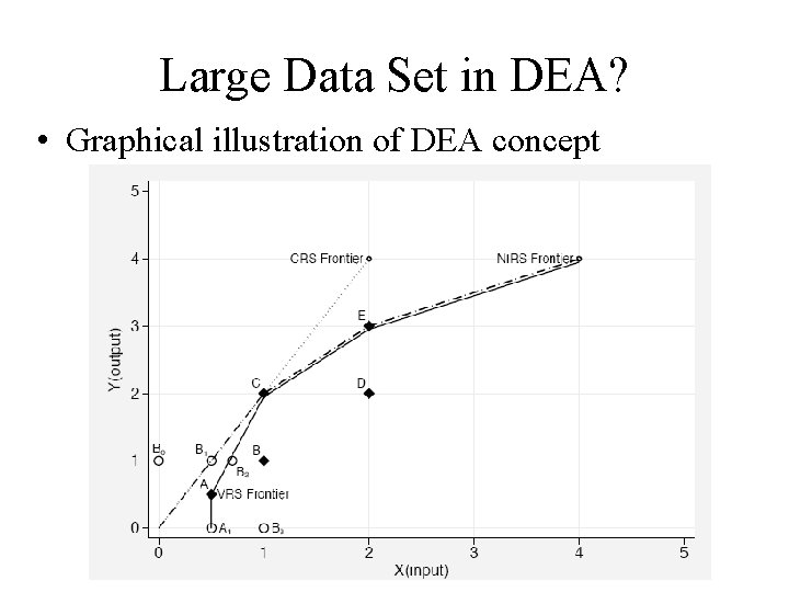
Large Data Set in DEA? • Graphical illustration of DEA concept

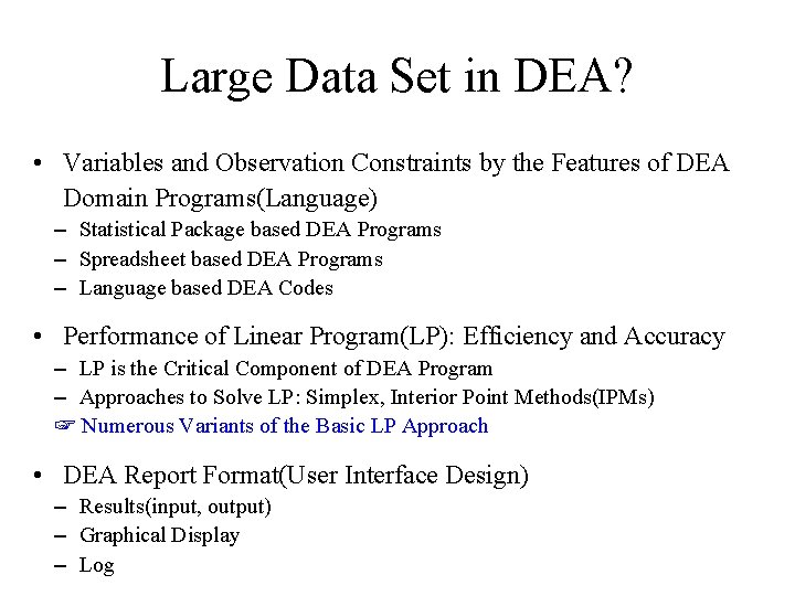
Large Data Set in DEA? • Variables and Observation Constraints by the Features of DEA Domain Programs(Language) – Statistical Package based DEA Programs – Spreadsheet based DEA Programs – Language based DEA Codes • Performance of Linear Program(LP): Efficiency and Accuracy – LP is the Critical Component of DEA Program – Approaches to Solve LP: Simplex, Interior Point Methods(IPMs) ☞ Numerous Variants of the Basic LP Approach • DEA Report Format(User Interface Design) – Results(input, output) – Graphical Display – Log

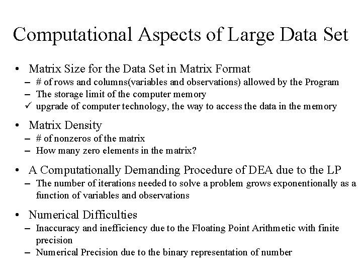
Computational Aspects of Large Data Set • Matrix Size for the Data Set in Matrix Format – # of rows and columns(variables and observations) allowed by the Program – The storage limit of the computer memory ü upgrade of computer technology, the way to access the data in the memory • Matrix Density – # of nonzeros of the matrix – How many zero elements in the matrix? • A Computationally Demanding Procedure of DEA due to the LP – The number of iterations needed to solve a problem grows exponentionally as a function of variables and observations • Numerical Difficulties – Inaccuracy and inefficiency due to the Floating Point Arithmetic with finite precision – Numerical Precision due to the binary representation of number

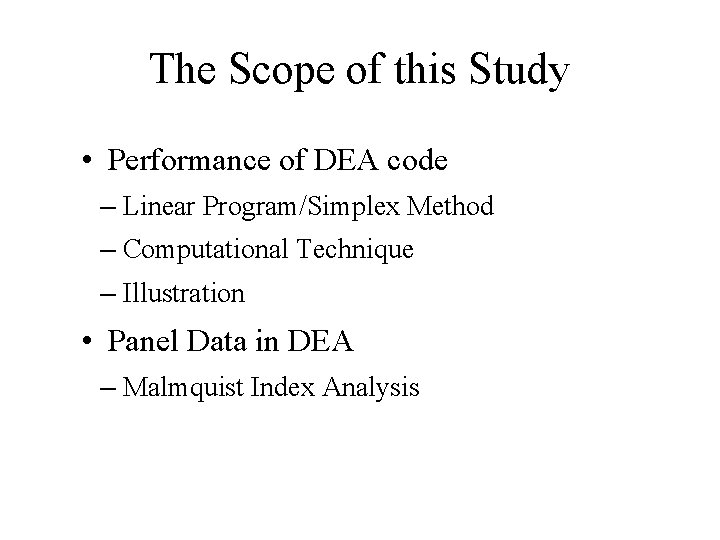
The Scope of this Study • Performance of DEA code – Linear Program/Simplex Method – Computational Technique – Illustration • Panel Data in DEA – Malmquist Index Analysis

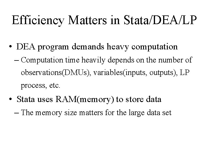
Efficiency Matters in Stata/DEA/LP • DEA program demands heavy computation – Computation time heavily depends on the number of observations(DMUs), variables(inputs, outputs), LP process, etc. • Stata uses RAM(memory) to store data – The memory size matters for the large data set

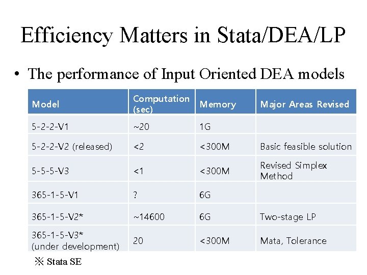
Efficiency Matters in Stata/DEA/LP • The performance of Input Oriented DEA models Model Computation (sec) Memory 5 -2 -2 -V 1 ~20 1 G 5 -2 -2 -V 2 (released) <2 <300 M Basic feasible solution 5 -5 -5 -V 3 <1 <300 M Revised Simplex Method 365 -1 -5 -V 1 ? 6 G 365 -1 -5 -V 2* ~14600 6 G Two-stage LP 365 -1 -5 -V 3* (under development) 20 <300 M Mata, Tolerance ※ Stata SE Major Areas Revised

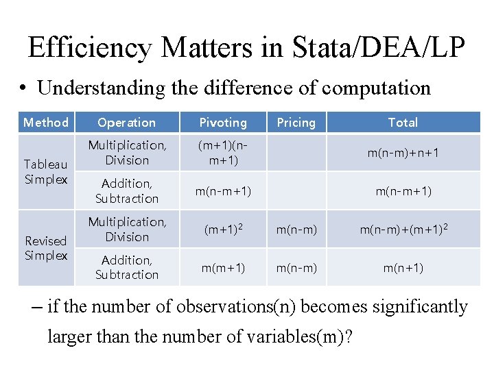
Efficiency Matters in Stata/DEA/LP • Understanding the difference of computation Method Tableau Simplex Revised Simplex Operation Pivoting Pricing Total Multiplication, Division (m+1)(nm+1) m(n-m)+n+1 Addition, Subtraction m(n-m+1) Multiplication, Division (m+1)2 m(n-m)+(m+1)2 Addition, Subtraction m(m+1) m(n-m) m(n+1) – if the number of observations(n) becomes significantly larger than the number of variables(m)?

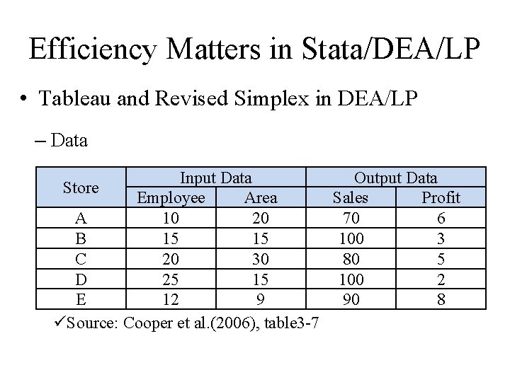
Efficiency Matters in Stata/DEA/LP • Tableau and Revised Simplex in DEA/LP – Data Input Data Output Data Store Employee Area Sales Profit A 10 20 70 6 B 15 15 100 3 C 20 30 80 5 D 25 15 100 2 E 12 9 90 8 üSource: Cooper et al. (2006), table 3 -7

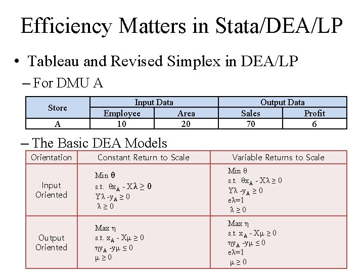
Efficiency Matters in Stata/DEA/LP • Tableau and Revised Simplex in DEA/LP – For DMU A Store A Input Data Employee Area 10 20 Output Data Sales Profit 70 6 – The Basic DEA Models Orientation Constant Return to Scale Variable Returns to Scale Input Oriented Min θ s. t. θx. A - Xλ ≥ 0 Yλ -y. A ≥ 0 λ≥ 0 Min θ s. t. θx. A - Xλ ≥ 0 Yλ -y. A ≥ 0 eλ=1 λ≥ 0 Output Oriented Max η s. t. x. A - Xμ ≥ 0 ηy. A -yμ ≤ 0 μ≥ 0 Max η s. t. x. A - Xμ ≥ 0 ηy. A -yμ ≤ 0 eλ=1 μ≥ 0

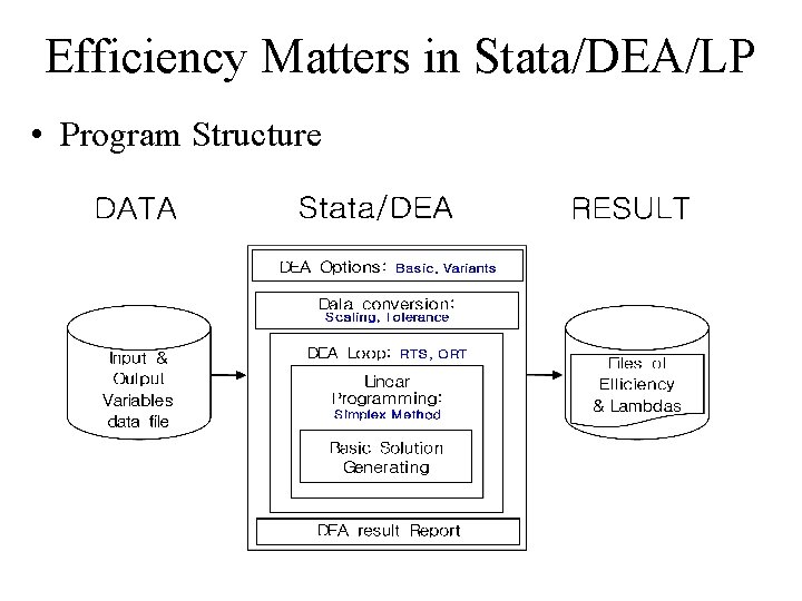
Efficiency Matters in Stata/DEA/LP • Program Structure

Efficiency Matters in Stata/DEA/LP • Program Syntax dea ivars = ovars [�if] � [�in] � [�, rts(cr out) stage(1 | 2) trace saving(filename)] – rts(crs | vrs | drs | irs) specifies the returns to scale. The default, rts(crs), specifies constant returns to scale. – ort(in | out) specifies the orientation. The default is ort(in), meaning input-oriented DEA. – stage(1 | 2) specifies the way to identify all efficiency slacks. The default is stage(2), meaning two-stage DEA. – trace specifies to save all the sequences displayed in the Results window in the dea. log file. The default is to save the final results in the dea. log file. – saving(filename) specifies that the results be saved in filename. dta.

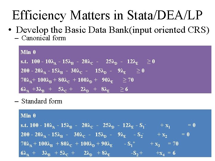
Efficiency Matters in Stata/DEA/LP • Develop the Basic Data Bank(input oriented CRS) – Canonical form Min θ s. t. 10θ - 10λA - 15λB - 20λC 20θ - 20λA - 15λB - 30λC - 25λD - 12λE 15λD - 70λA+ 100λB + 80λC + 100λD + 90λE 6λA +3λB + 5λC + 2λD + 8λE 9λE ≥ 0 ≥ 70 ≥ 6 – Standard form Min θ s. t. 10θ - 10λA - 15λB - 20λC - 25λD - 12λE - S 120θ - 20λA - 15λB - 30λC - 15λD - 70λA + 100λB + 80λC + 100λD + 90λE 6λA + 3λB + 5λC + 2λD + 8λE 9λE - S 2 - - S 1 + -S 2 + + x 1 + x 2 + x 3 =0 =0 = 70 +x 4 = 6

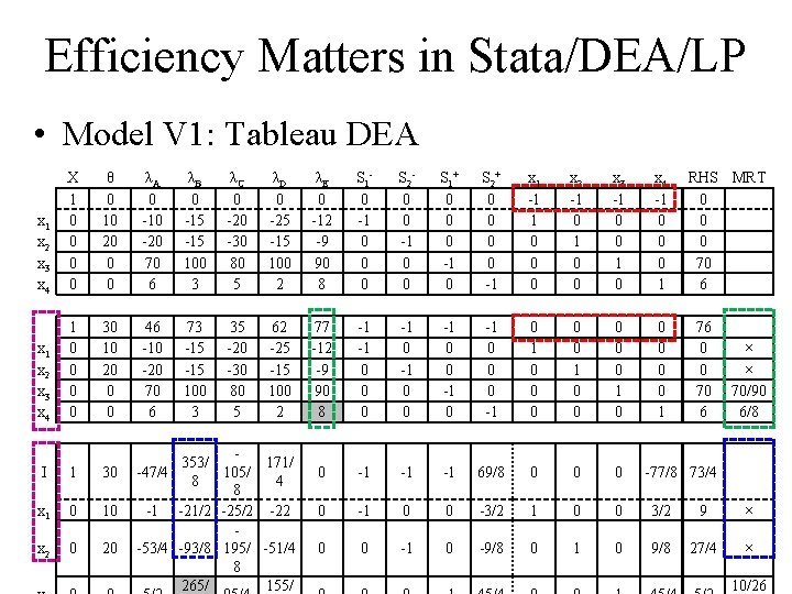
Efficiency Matters in Stata/DEA/LP • Model V 1: Tableau DEA x 1 x 2 x 3 x 4 X 1 0 0 θ 0 10 20 0 0 λA 0 -10 -20 70 6 λB 0 -15 100 3 λC 0 -20 -30 80 5 λD 0 -25 -15 100 2 λE 0 -12 -9 90 8 S 1 0 -1 0 0 0 S 2 0 0 -1 0 0 S 1 + 0 0 0 -1 0 S 2 + 0 0 -1 x 1 -1 1 0 0 0 x 2 -1 0 0 x 3 -1 0 0 1 0 x 4 -1 0 0 0 1 x 2 x 3 x 4 1 0 0 30 10 20 0 0 46 -10 -20 70 6 73 -15 100 3 35 -20 -30 80 5 62 -25 -15 100 2 77 -12 -9 90 8 -1 -1 0 0 0 -1 0 -1 0 0 0 0 0 1 0 -1 -1 -1 69/8 0 0 -1 0 0 -3/2 1 0 0 3/2 9 × 0 0 -1 0 -9/8 0 1 0 9/8 27/4 × Ⅰ 1 30 x 1 0 10 x 2 0 20 353/ 171/ 105/ -47/4 8 -1 -21/2 -25/2 -22 -53/4 -93/8 195/ -51/4 8 265/ 155/ RHS MRT 0 0 0 70 6 76 0 0 70 6 × × 70/90 6/8 -77/8 73/4 10/26

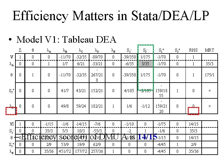
Efficiency Matters in Stata/DEA/LP • Model V 1: Tableau DEA Z θ λA λB λC λD λE S 1 - S 2 - S 1 + S 2 + RHS Ⅴ 1 0 0 -11/70 -32/35 -89/70 0 -39/350 1/175 -1/70 0 1 λA 0 0 1 1/7 6/21 0 -6/35 3/35 -1/70 0 1 35/3 θ 0 1 0 -11/70 -32/35 -33/21 267/21 0 0 -39/350 1/175 -1/70 0 1 175/1 1 0 × 0 0 × S 2 159/18 55 159/21 20 + 0 0 0 41/7 43/21 152/21 0 4/105 -2/105 λE 0 0 0 49/8 59/24 182/21 1 1/6 -1/12 Ⅵ 1 0 -1/15 -1/6 -14/15 -7/6 0 -1/10 0 -1/75 0 14/15 S 2 - 0 0 35/3 10/3 -55/3 0 -2 1 -1/6 0 35/3 0 14/15 θ 1 -1/15 score(θ) -1/6 -14/15 of -7/6 DMU 0 0 -1/15 – 0 Efficiency A-1/10 is 14/15 S 2 + 0 0 2/9 λE 0 0 35/36 53/9 19/9 62/9 451/72 177/72 257/36 0 0 0 -4/45 1 2/9 1 0 0 -4/45 0 35/36 MRT

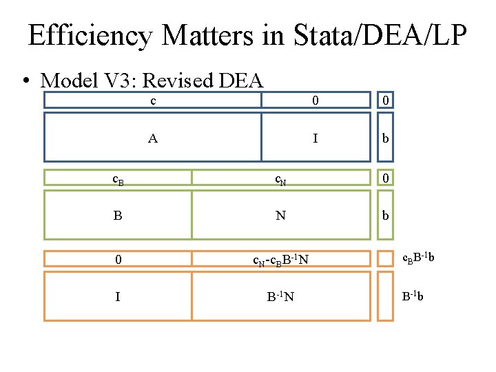
Efficiency Matters in Stata/DEA/LP • Model V 3: Revised DEA c 0 0 A I b c. B c. N 0 B N b 0 c. N-c. BB-1 N I B-1 N c. BB-1 b

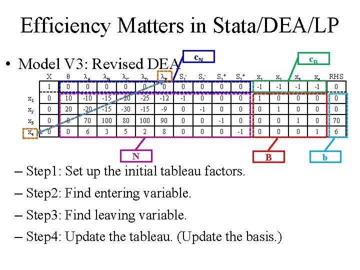
Efficiency Matters in Stata/DEA/LP c. N • Model V 3: Revised DEA c. B X 1 θ 0 λA 0 λB 0 λC 0 λD 0 λE 0 S 1 0 S 2 0 S 1 + 0 S 2 + 0 x 1 -1 x 2 -1 x 3 -1 x 4 -1 RHS 0 x 1 0 10 -15 -20 -25 -12 -1 0 0 0 0 x 2 0 20 -15 -30 -15 -9 0 -1 0 0 0 x 3 0 0 70 100 80 100 90 0 0 -1 0 0 0 1 0 70 x 4 0 0 6 3 5 2 8 0 0 0 -1 0 0 0 1 6 N B – Step 1: Set up the initial tableau factors. – Step 2: Find entering variable. – Step 3: Find leaving variable. – Step 4: Update the tableau. (Update the basis. ) b

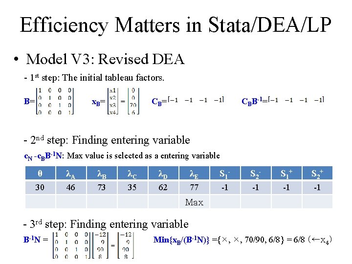
Efficiency Matters in Stata/DEA/LP • Model V 3: Revised DEA - 1 st step: The initial tableau factors. B= x. B= CBB-1= - 2 nd step: Finding entering variable c. N -c. BB-1 N: Max value is selected as a entering variable θ λA λB λC λD λE S 1 - S 2 - S 1 + S 2 + 30 46 73 35 62 77 -1 -1 Max - 3 rd step: Finding entering variable B-1 N = Min{x. B/(B-1 N)} ={×, ×, 70/90, 6/8} = 6/8 (←x 4)

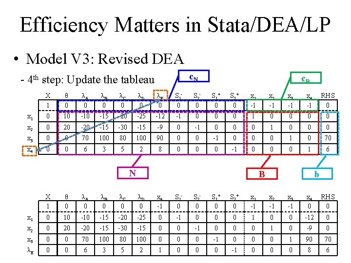
Efficiency Matters in Stata/DEA/LP • Model V 3: Revised DEA c. N - 4 th step: Update the tableau c. B X 1 θ 0 λA 0 λB 0 λC 0 λD 0 λE 0 S 1 0 S 2 0 S 1 + 0 S 2 + 0 x 1 -1 x 2 -1 x 3 -1 x 4 -1 RHS 0 x 1 0 10 -15 -20 -25 -12 -1 0 0 0 0 x 2 0 20 -15 -30 -15 -9 0 -1 0 0 0 x 3 0 0 70 100 80 100 90 0 0 -1 0 0 0 1 0 70 x 4 0 0 6 3 5 2 8 0 0 0 -1 0 0 0 1 6 N B b X 1 θ 0 λA 0 λB 0 λC 0 λD 0 x 4 -1 S 1 0 S 2 0 S 1 + 0 S 2 + 0 x 1 -1 x 2 -1 x 3 -1 x 4 0 RHS 0 x 1 0 10 -15 -20 -25 0 -1 0 0 0 1 0 0 -12 0 x 2 0 20 -15 -30 -15 0 0 -1 0 0 0 1 0 -9 0 x 3 0 0 70 100 80 100 0 -1 0 0 0 1 90 70 λE 0 0 6 3 5 2 1 0 0 0 -1 0 0 0 8 6

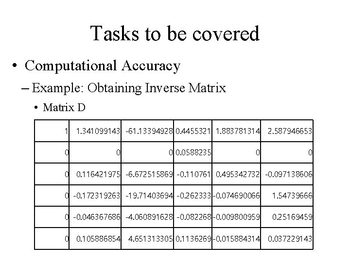
Tasks to be covered • Computational Accuracy – Example: Obtaining Inverse Matrix • Matrix D 1 1. 341099143 -61. 13394928 0. 4455321 1. 883781314 0 0. 0588235 0 2. 587946653 0 0 0. 116421975 -6. 672515869 -0. 110761 0. 495342732 -0. 097138606 0 -0. 172319263 -19. 71403694 -0. 262333 -0. 074690066 1. 54739666 0 -0. 046367686 -4. 060891628 -0. 082268 -0. 009800959 0. 25169459 0 0. 105886854 4. 651313305 0. 1136269 -0. 015884314 0. 037229143

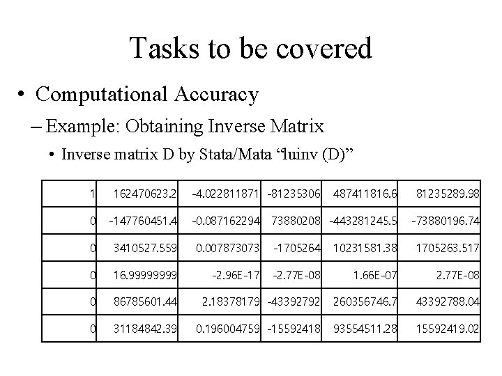
Tasks to be covered • Computational Accuracy – Example: Obtaining Inverse Matrix • Inverse matrix D by Stata/Mata “luinv (D)” 1 162470623. 2 -4. 022811871 -81235306 487411816. 6 81235289. 98 0 -147760451. 4 -0. 087162294 73880208 -443281245. 5 -73880196. 74 0 3410527. 559 0. 007873073 -1705264 10231581. 38 1705263. 517 0 16. 9999 -2. 96 E-17 -2. 77 E-08 1. 66 E-07 2. 77 E-08 0 86785601. 44 2. 18378179 -43392792 260356746. 7 43392788. 04 0 31184842. 39 0. 196004759 -15592418 93554511. 28 15592419. 02

Tasks to be covered • Computational Accuracy – Example: Obtaining Inverse Matrix • Inverse matrix D by Stata/Mata “luinv (D)”

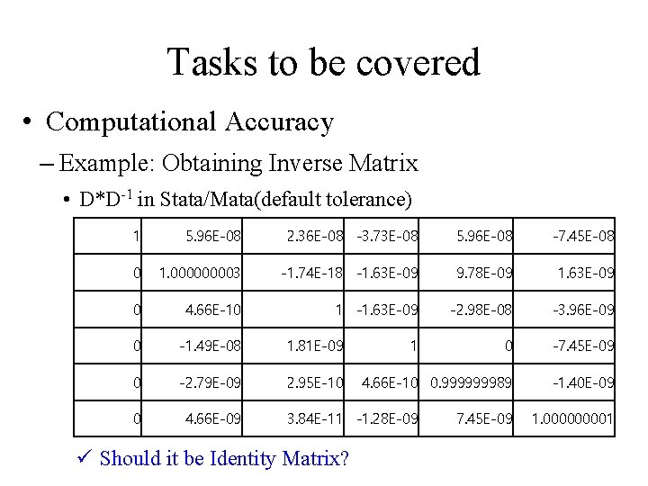
Tasks to be covered • Computational Accuracy – Example: Obtaining Inverse Matrix • D*D-1 in Stata/Mata(default tolerance) 1 5. 96 E-08 2. 36 E-08 -3. 73 E-08 5. 96 E-08 -7. 45 E-08 0 1. 00003 -1. 74 E-18 -1. 63 E-09 9. 78 E-09 1. 63 E-09 0 4. 66 E-10 1 -1. 63 E-09 -2. 98 E-08 -3. 96 E-09 0 -1. 49 E-08 1. 81 E-09 0 -7. 45 E-09 0 -2. 79 E-09 2. 95 E-10 4. 66 E-10 0. 999999989 -1. 40 E-09 0 4. 66 E-09 1 3. 84 E-11 -1. 28 E-09 ü Should it be Identity Matrix? 7. 45 E-09 1. 00001

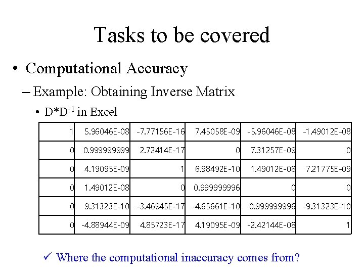
Tasks to be covered • Computational Accuracy – Example: Obtaining Inverse Matrix • D*D-1 in Excel 1 5. 96046 E-08 -7. 77156 E-16 0 0. 99999 2. 72414 E-17 0 7. 31257 E-09 0 0 4. 19095 E-09 1 6. 98492 E-10 1. 49012 E-08 7. 21775 E-09 0 1. 49012 E-08 0 0. 99996 0 0 0 9. 31323 E-10 -3. 46945 E-17 -4. 65661 E-10 0 -4. 88944 E-09 4. 85723 E-17 7. 45058 E-09 -5. 96046 E-08 -1. 49012 E-08 0. 99996 -9. 31323 E-10 4. 19095 E-09 -2. 42144 E-08 ü Where the computational inaccuracy comes from? 1

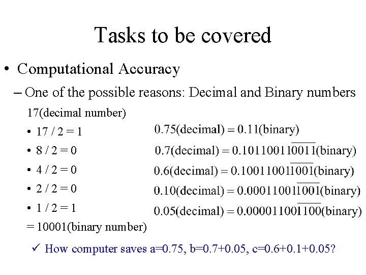
Tasks to be covered • Computational Accuracy – One of the possible reasons: Decimal and Binary numbers 17(decimal number) • 17 / 2 = 1 • 8/2=0 • 4/2=0 • 2/2=0 • 1/2=1 = 10001(binary number) ü How computer saves a=0. 75, b=0. 7+0. 05, c=0. 6+0. 1+0. 05?

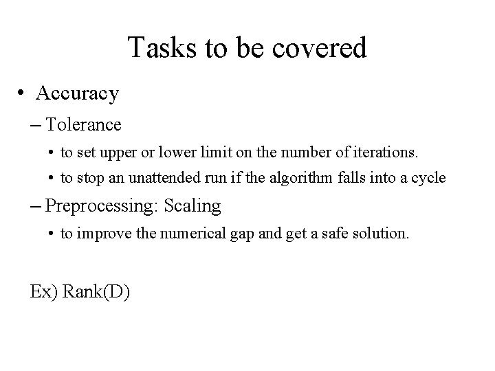
Tasks to be covered • Accuracy – Tolerance • to set upper or lower limit on the number of iterations. • to stop an unattended run if the algorithm falls into a cycle – Preprocessing: Scaling • to improve the numerical gap and get a safe solution. Ex) Rank(D)

Part II. Malmquist Index Analysis with the Panel Data Basic Concept of Malmquist Index The User Written Command “malmq”

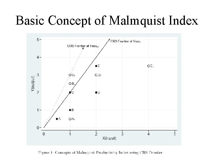
Basic Concept of Malmquist Index • Malmquist Productivity Index(MPI) measures the productivity changes along with time variations and can be decomposed into changes in efficiency and technology.

Basic Concept of Malmquist Index

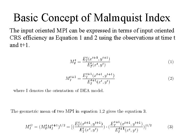
Basic Concept of Malmquist Index The input oriented MPI can be expressed in terms of input oriented CRS efficiency as Equation 1 and 2 using the observations at time t and t+1.

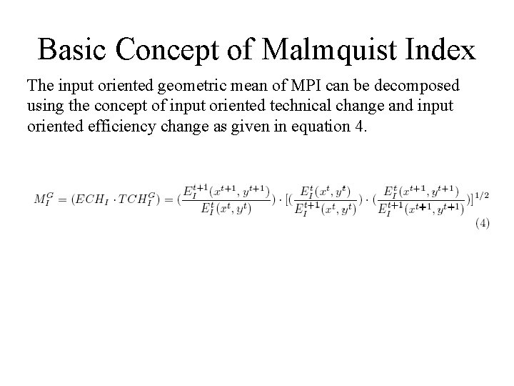
Basic Concept of Malmquist Index The input oriented geometric mean of MPI can be decomposed using the concept of input oriented technical change and input oriented efficiency change as given in equation 4.

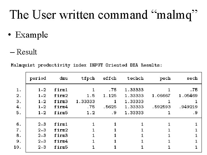
The User written command “malmq” • Program Syntax malmq ivars = ovars [�if] � [�in] � [�, ort( period(varname) trace saving(filename)] – ort(in | out) specifies the orientation. The default is ort(in), meaning input-oriented DEA. – period(varname) identifies the time variable. – trace specifies to save all the sequences displayed in the Results window in the malmq. log file. The default is to save the final results in the malmq. log file. – saving(filename) specifies that the results be saved in filename. dta.

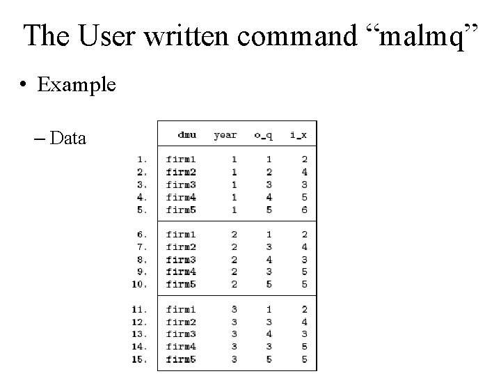
The User written command “malmq” • Example – Data

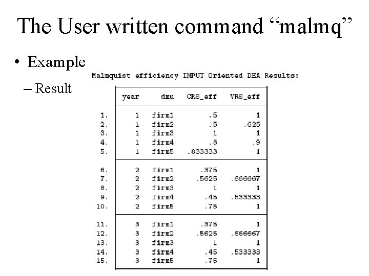
The User written command “malmq” • Example – Result

The User written command “malmq” • Example – Result

Notes • The data and code related to the presentation will be available from the Conference website.

References • Cooper, W. W. , Seiford, L. M. , & Tone, A. (2006). Introduction to Data Envelopment Analysis and Its Uses, Springer Science+Business Media. • Ji, Y. , & Lee, C. (2010). “Data Envelopment Analysis”, The Stata Journal, 10(no. 2), pp. 267 -280. • Lee, C. , & Ji, Y. (2009). “Data Envelopment Analysis in Stata”, DC 09 Stata Conference. • Maros, Istvan. (2003). Computational techniques of the simplex method, Kluwer Academic Publishers.