Advances in LAM 3 DVAR formulation Vincent GUIDARD

Advances in LAM 3 D-VAR formulation Vincent GUIDARD Claude FISCHER Météo-France, CNRM/GMAP

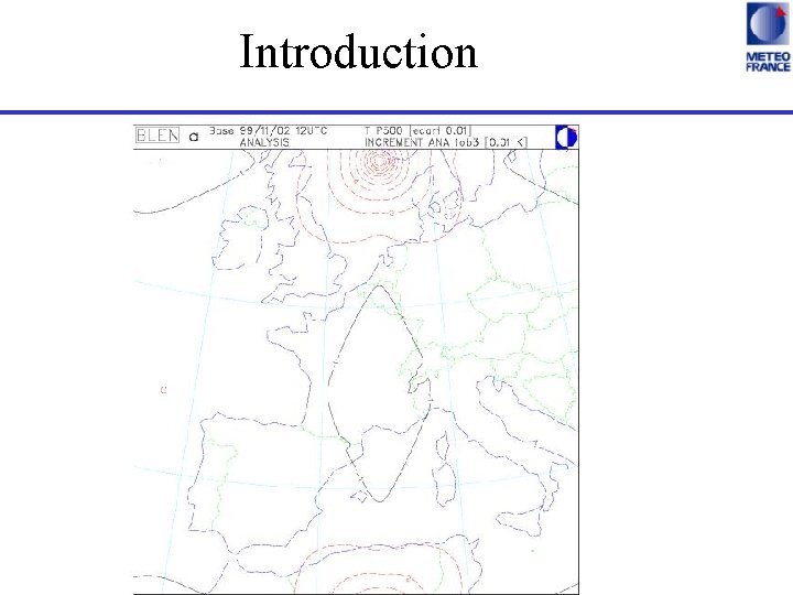
Introduction • Through various experiments, a drawback of biperiodic increments has arisen : « wrapping around » analysis increments

Introduction

Introduction • Through various experiments, a drawback of biperiodic increments has arisen: « wrapping around » analysis increments Controlling the lengthscale of the correlation functions is necessary: compact support • Introduction of a large-scale information in the LAM analysis to let the increments due to the observations be of mesoscale

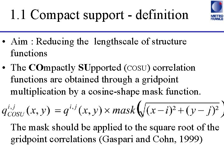
1. 1 Compact support - definition • Aim : Reducing the lengthscale of structure functions • The COmpactly SUpported (COSU) correlation functions are obtained through a gridpoint multiplication by a cosine-shape mask function. The mask should be applied to the square root of the gridpoint correlations (Gaspari and Cohn, 1999)

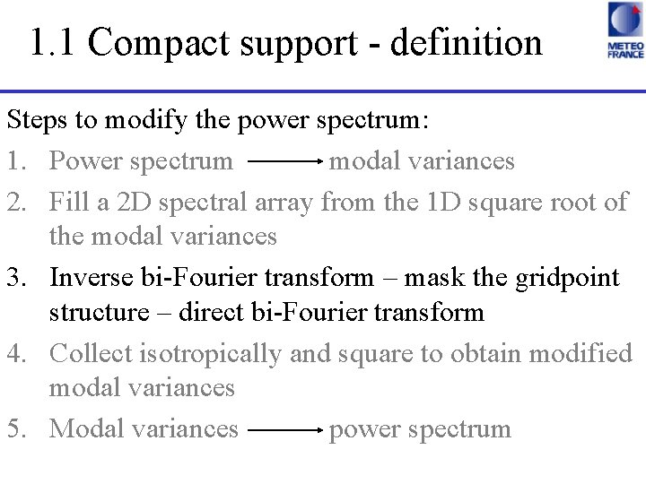
1. 1 Compact support - definition Steps to modify the power spectrum: 1. Power spectrum modal variances 2. Fill a 2 D spectral array from the 1 D square root of the modal variances 3. Inverse bi-Fourier transform – mask the gridpoint structure – direct bi-Fourier transform 4. Collect isotropically and square to obtain modified modal variances 5. Modal variances power spectrum

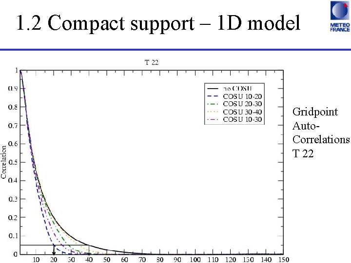
1. 2 Compact support – 1 D model Gridpoint Auto. Correlations T 22

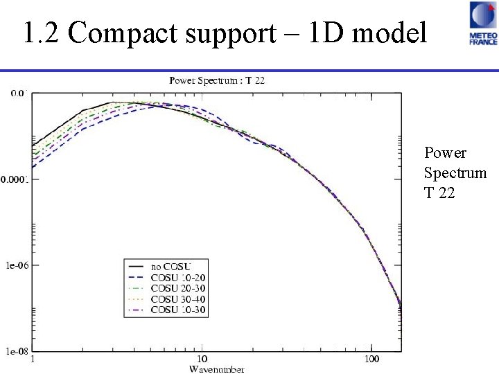
1. 2 Compact support – 1 D model Power Spectrum T 22

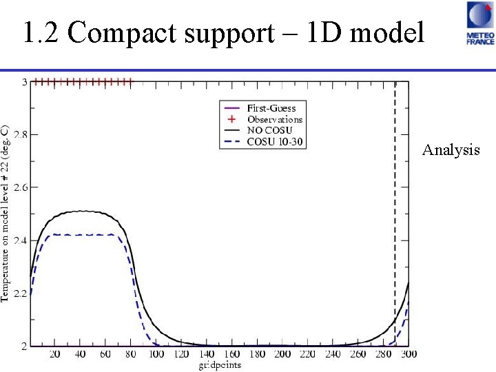
1. 2 Compact support – 1 D model Analysis

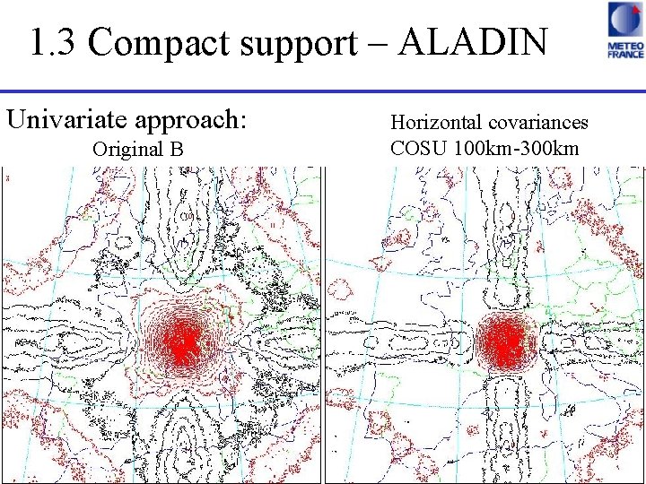
1. 3 Compact support – ALADIN Univariate approach: Original B Horizontal covariances COSU 100 km-300 km

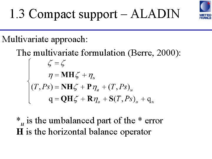
1. 3 Compact support – ALADIN Multivariate approach: The multivariate formulation (Berre, 2000): *u is the umbalanced part of the * error H is the horizontal balance operator

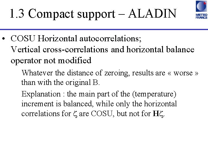
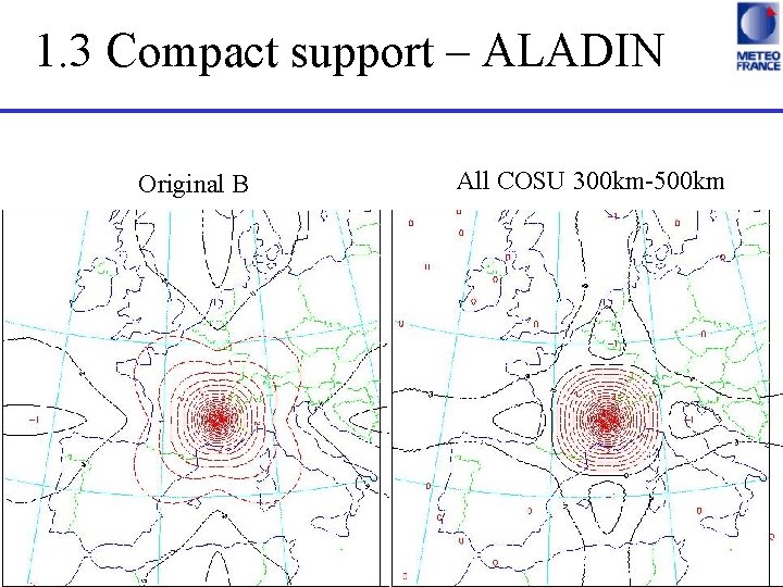
1. 3 Compact support – ALADIN • COSU Horizontal autocorrelations; Vertical cross-correlations and horizontal balance operator not modified Whatever the distance of zeroing, results are « worse » than with the original B. Explanation : the main part of the (temperature) increment is balanced, while only the horizontal correlations for z are COSU, but not for Hz.

1. 3 Compact support – ALADIN – Cure 1: a modification of the z power spectrum in order to have COSU correlations for Hz same results as the original B. – Cure 2: another solution is to compactly support the horizontal balance operator

1. 3 Compact support – ALADIN Original B All COSU 300 km-500 km

1. 3 Compact support – conclusion • Single observation: – Very efficient technique in univariate case – Needs drastic measures (COSU horizontal balance) to be efficient in multivariate case • Full observation set: – No impact, even with drastic measures – Further research is necessary – Problems possibly due to a large scale error which this mesoscale analysis tries to reduce use of another source of information for large scales

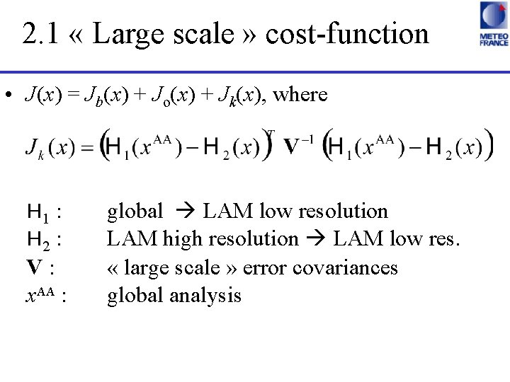
2. 1 « Large scale » cost-function • Aim : input a large scale information in the LAM 3 D-VAR. • The large scale information is the analysis of the global model (ARPEGE) put to a LAM low resolution geometry • Thanks to classical hypotheses, plus assuming that the global analysis error and the LAM background error are NOT correlated, we simply add a new term to the cost function

2. 1 « Large scale » cost-function • J(x) = Jb(x) + Jo(x) + Jk(x), where H 1 : H 2 : V: x. AA : global LAM low resolution LAM high resolution LAM low res. « large scale » error covariances global analysis

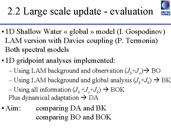
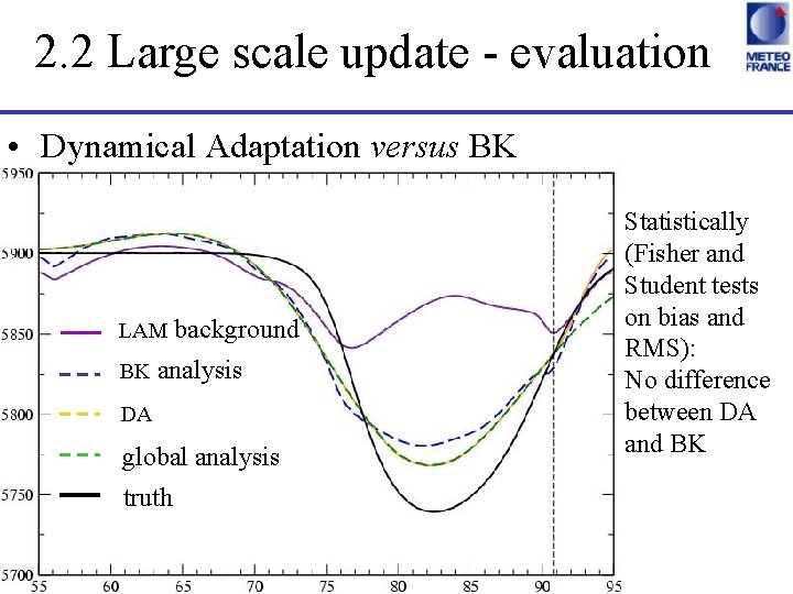
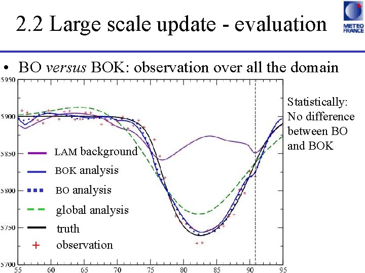
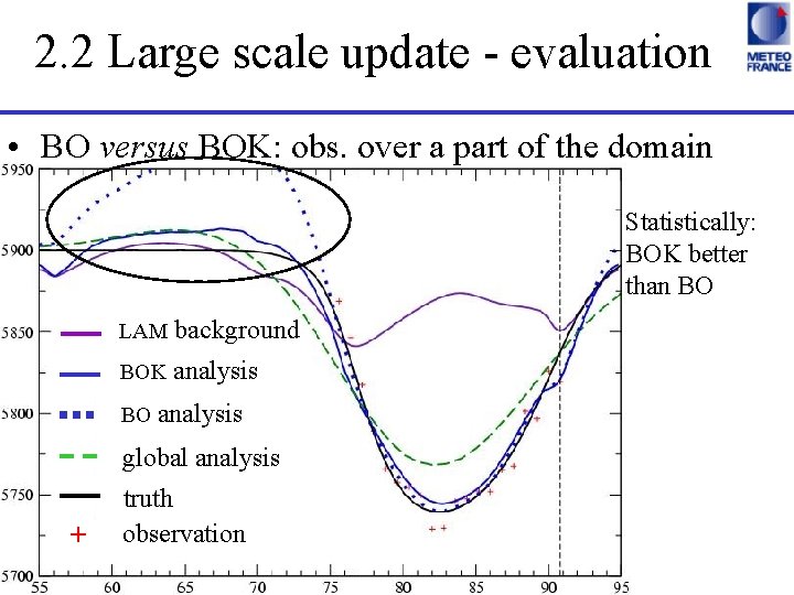
2. 2 Large scale update - evaluation • 1 D Shallow Water « global » model (I. Gospodinov) LAM version with Davies coupling (P. Termonia) Both spectral models • 1 D gridpoint analyses implemented: – Using LAM background and observation (Jb+Jo) BO – Using LAM background and global analysis (Jb+Jk) BK – Using all information (Jb +Jo+Jk) BOK Plus dynamical adaptation DA • Aim: comparing DA and BK comparing BO and BOK

2. 2 Large scale update - evaluation • Dynamical Adaptation versus BK LAM BK background analysis DA global analysis truth Statistically (Fisher and Student tests on bias and RMS): No difference between DA and BK

2. 2 Large scale update - evaluation • BO versus BOK: observation over all the domain LAM background BOK analysis BO analysis global analysis + truth observation Statistically: No difference between BO and BOK

2. 2 Large scale update - evaluation • BO versus BOK: obs. over a part of the domain Statistically: BOK better than BO LAM background BOK analysis BO analysis global analysis + truth observation

2. 3 Large scale update - conclusion • The large scale information seems useful only in border-line cases, in the Shallow Water model • Next steps : – Evaluation in a Burger model – Ensemble evaluation of the statistics in ARPEGEALADIN (based on the work of Loïk Berre, Margarida Belo-Pereira and Simona Stefanescu) – Implementation in ALADIN