A MAXENT viewpoint 600 465 Intro to NLP

A MAXENT viewpoint 600. 465 - Intro to NLP - J. Eisner 1

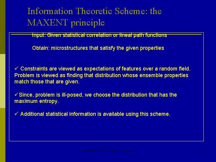
Information Theoretic Scheme: the MAXENT principle Input: Given statistical correlation or lineal path functions Obtain: microstructures that satisfy the given properties ü Constraints are viewed as expectations of features over a random field. Problem is viewed as finding that distribution whose ensemble properties match those that are given. üSince, problem is ill-posed, we choose the distribution that has the maximum entropy. ü Additional statistical information is available using this scheme. 600. 465 - Intro to NLP - J. Eisner 2

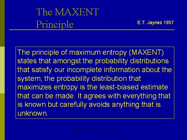
The MAXENT Principle E. T. Jaynes 1957 The principle of maximum entropy (MAXENT) states that amongst the probability distributions that satisfy our incomplete information about the system, the probability distribution that maximizes entropy is the least-biased estimate that can be made. It agrees with everything that is known but carefully avoids anything that is unknown. 600. 465 - Intro to NLP - J. Eisner 3

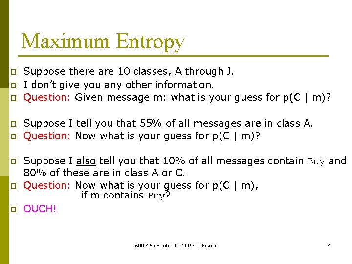
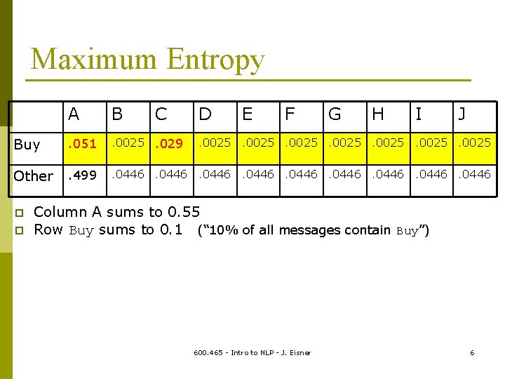
Maximum Entropy p p p p Suppose there are 10 classes, A through J. I don’t give you any other information. Question: Given message m: what is your guess for p(C | m)? Suppose I tell you that 55% of all messages are in class A. Question: Now what is your guess for p(C | m)? Suppose I also tell you that 10% of all messages contain Buy and 80% of these are in class A or C. Question: Now what is your guess for p(C | m), if m contains Buy? OUCH! 600. 465 - Intro to NLP - J. Eisner 4

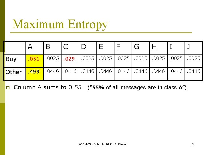
Maximum Entropy A B Buy . 051 . 0025. 029 Other . 499 . 0446 p C D E F G H I J . 0025 Column A sums to 0. 55 (“ 55% of all messages are in class A”) 600. 465 - Intro to NLP - J. Eisner 5

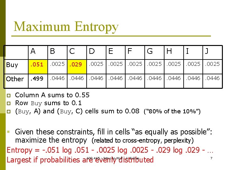
Maximum Entropy A B Buy . 051 . 0025. 029 Other . 499 . 0446 p p C D E F G H I J . 0025 Column A sums to 0. 55 Row Buy sums to 0. 1 (“ 10% of all messages contain Buy”) 600. 465 - Intro to NLP - J. Eisner 6

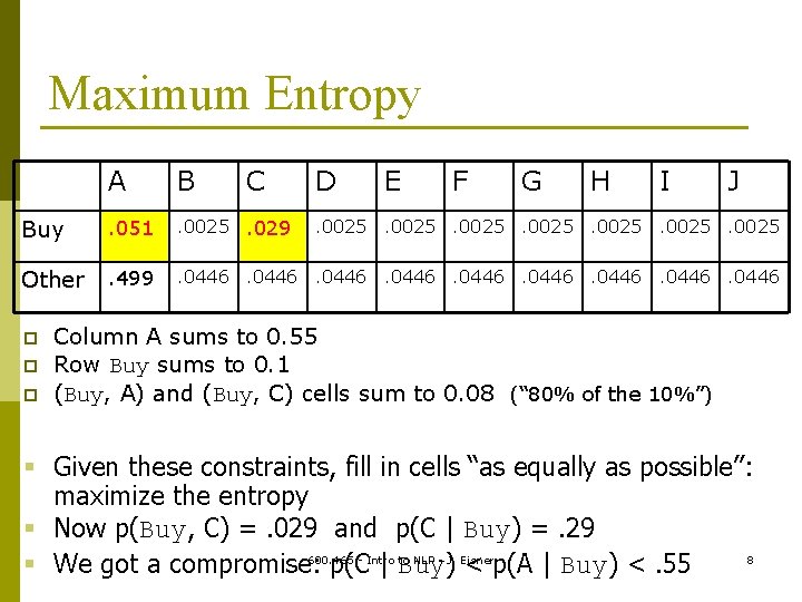
Maximum Entropy A B Buy . 051 . 0025. 029 Other . 499 . 0446 p p p C D E F G H I J . 0025 Column A sums to 0. 55 Row Buy sums to 0. 1 (Buy, A) and (Buy, C) cells sum to 0. 08 (“ 80% of the 10%”) § Given these constraints, fill in cells “as equally as possible”: maximize the entropy (related to cross-entropy, perplexity) Entropy = -. 051 log. 051 -. 0025 log. 0025 -. 029 log. 029 - … 600. 465 - Intro to NLP - J. Eisner 7 Largest if probabilities are evenly distributed

Maximum Entropy A B Buy . 051 . 0025. 029 Other . 499 . 0446 p p p C D E F G H I J . 0025 Column A sums to 0. 55 Row Buy sums to 0. 1 (Buy, A) and (Buy, C) cells sum to 0. 08 (“ 80% of the 10%”) § Given these constraints, fill in cells “as equally as possible”: maximize the entropy § Now p(Buy, C) =. 029 and p(C | Buy) =. 29 600. 465 - Intro to NLP - J. Eisner 8 § We got a compromise: p(C | Buy) < p(A | Buy) <. 55

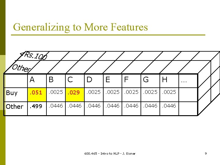
Generalizing to More Features <Rs. 10 0 Other A B C D E F G H Buy . 051 . 0025. 029 Other . 499 . 0446 … . 0025 600. 465 - Intro to NLP - J. Eisner 9

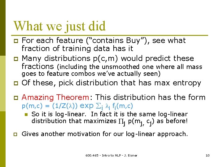
What we just did p p For each feature (“contains Buy”), see what fraction of training data has it Many distributions p(c, m) would predict these fractions (including the unsmoothed one where all mass goes to feature combos we’ve actually seen) p Of these, pick distribution that has max entropy p Amazing Theorem: This distribution has the form p(m, c) = (1/Z( )) exp i i fi(m, c) n p So it is log-linear. In fact it is the same log-linear distribution that maximizes j p(mj, cj) as before! Gives another motivation for our log-linear approach. 600. 465 - Intro to NLP - J. Eisner 10

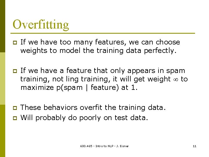
Overfitting p If we have too many features, we can choose weights to model the training data perfectly. p If we have a feature that only appears in spam training, not ling training, it will get weight to maximize p(spam | feature) at 1. p These behaviors overfit the training data. Will probably do poorly on test data. p 600. 465 - Intro to NLP - J. Eisner 11

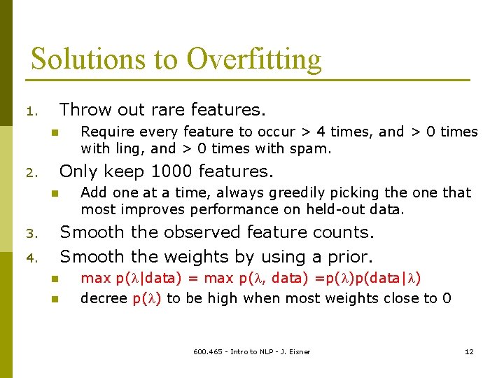
Solutions to Overfitting Throw out rare features. 1. n Require every feature to occur > 4 times, and > 0 times with ling, and > 0 times with spam. Only keep 1000 features. 2. n Add one at a time, always greedily picking the one that most improves performance on held-out data. Smooth the observed feature counts. Smooth the weights by using a prior. 3. 4. n n max p( |data) = max p( , data) =p( )p(data| ) decree p( ) to be high when most weights close to 0 600. 465 - Intro to NLP - J. Eisner 12