4 2 kconnected graphs This copyrighted material is

4. 2 k-connected graphs This copyrighted material is taken from Introduction to Graph Theory, 2 nd Ed. , by Doug West; and is not for further distribution beyond this course. These slides will be stored in a limited-access location on an IIT server and are not for distribution or use beyond Math 454/553. 1

No Loops in Chapter 4 For all of Chapter 4, graphs have no loops. This applies to the statements and proofs of all results. 2

3 Extended characterization for 2 -connectedness 4. 2. 4 Theorem. Let a graph G have 3 vertices. The following are equivalent (TFAE): (A) G is connected and has no cut-vertex; (B) For all x, y V(G), there exist internally disjoint x, y-paths; (C) For all x, y V(G), there is a cycle through x and y; and (D) (G) 1, and every pair of edges lies on a common cycle. Proof. (A) <=> (B) is by Thm. 4. 2. 2. (B) <=> (C) P u C=P Q cycle iff two disjoint paths Q Contains copyrighted material from Introduction to Graph Theory by Doug West, 2 nd Ed. Not for distribution beyond IIT’s Math 454/553. v

4. 2 Extended characterization for 2 -connectedness (D)<=>(C): ( (G) 1, any 2 edges are in some same cycle <=> any 2 vertices are in some same cycle) Let x, y V(G). Min degree forces each incident to an edge: x y ? z y Case 1 x<->y x n(G)¸ 3, so there is a third vertex z. A cycle through these two edges also goes through x, y. x ? ? y Case 2 x<->y A cycle through these two edges also goes through x, y. Contains copyrighted material from Introduction to Graph Theory by Doug West, 2 nd Ed. Not for distribution beyond IIT’s Math 454/553. 4

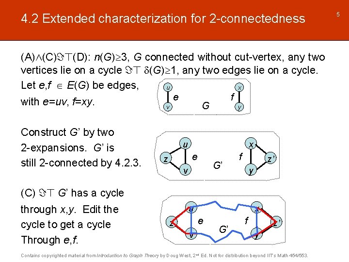
4. 2 Extended characterization for 2 -connectedness (A)^(C)=>(D): n(G) 3, G connected without cut-vertex, any two vertices lie on a cycle => (G) 1, any two edges lie on a cycle. Let e, f E(G) be edges, u x with e=uv, f=xy. Construct G’ by two 2 -expansions. G’ is still 2 -connected by 4. 2. 3. e f G v y u x e z G’ v f z’ y (C) => G’ has a cycle through x, y. Edit the cycle to get a cycle Through e, f. u x e z v G’ f z’ y Contains copyrighted material from Introduction to Graph Theory by Doug West, 2 nd Ed. Not for distribution beyond IIT’s Math 454/553. 5

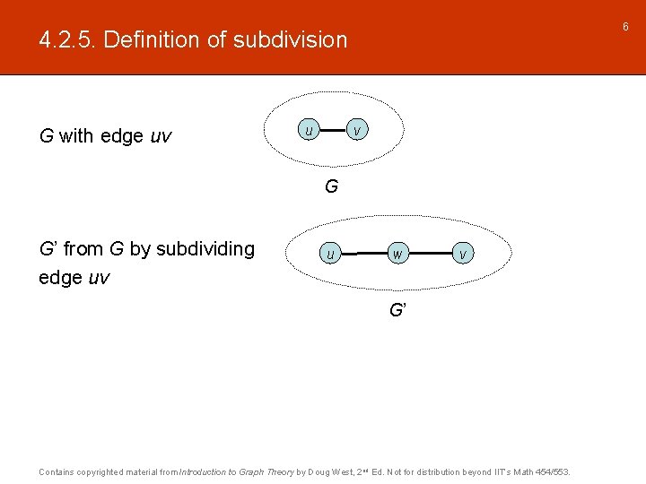
6 4. 2. 5. Definition of subdivision G with edge uv u v G G’ from G by subdividing edge uv u w v G’ Contains copyrighted material from Introduction to Graph Theory by Doug West, 2 nd Ed. Not for distribution beyond IIT’s Math 454/553.

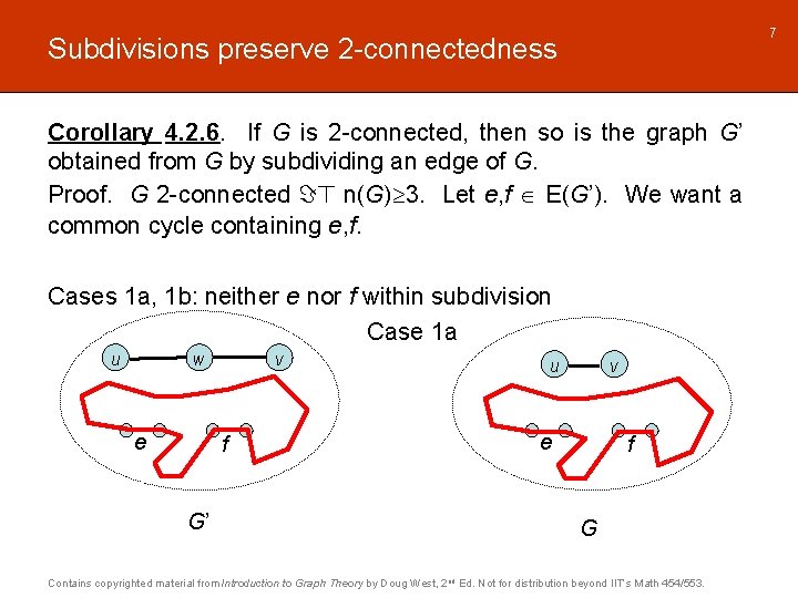
7 Subdivisions preserve 2 -connectedness Corollary 4. 2. 6. If G is 2 -connected, then so is the graph G’ obtained from G by subdividing an edge of G. Proof. G 2 -connected => n(G) 3. Let e, f E(G’). We want a common cycle containing e, f. Cases 1 a, 1 b: neither e nor f within subdivision Case 1 a u w e v f G’ u v e f G Contains copyrighted material from Introduction to Graph Theory by Doug West, 2 nd Ed. Not for distribution beyond IIT’s Math 454/553.

8 Subdivisions preserve 2 -connectedness Corollary 4. 2. 6. If G is 2 -connected, then so is the graph G’ obtained from G by subdividing an edge of G. Proof. G 2 -connected => n(G) 3. Let e, f E(G’). We want a common cycle containing e, f. Cases 1 a, 1 b: neither e nor f within subdivision Case 1 b u w e v f G’ u v e f G Contains copyrighted material from Introduction to Graph Theory by Doug West, 2 nd Ed. Not for distribution beyond IIT’s Math 454/553.

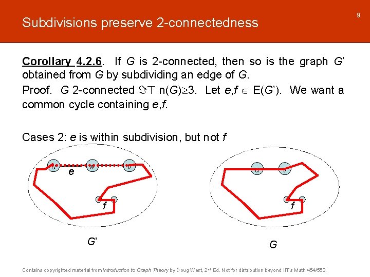
9 Subdivisions preserve 2 -connectedness Corollary 4. 2. 6. If G is 2 -connected, then so is the graph G’ obtained from G by subdividing an edge of G. Proof. G 2 -connected => n(G) 3. Let e, f E(G’). We want a common cycle containing e, f. Cases 2: e is within subdivision, but not f u e w v u v f G’ f G Contains copyrighted material from Introduction to Graph Theory by Doug West, 2 nd Ed. Not for distribution beyond IIT’s Math 454/553.

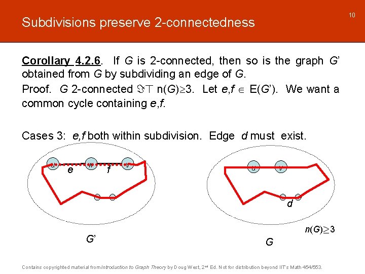
10 Subdivisions preserve 2 -connectedness Corollary 4. 2. 6. If G is 2 -connected, then so is the graph G’ obtained from G by subdividing an edge of G. Proof. G 2 -connected => n(G) 3. Let e, f E(G’). We want a common cycle containing e, f. Cases 3: e, f both within subdivision. Edge d must exist. u e w f v u v d G’ n(G)¸ 3 G Contains copyrighted material from Introduction to Graph Theory by Doug West, 2 nd Ed. Not for distribution beyond IIT’s Math 454/553.

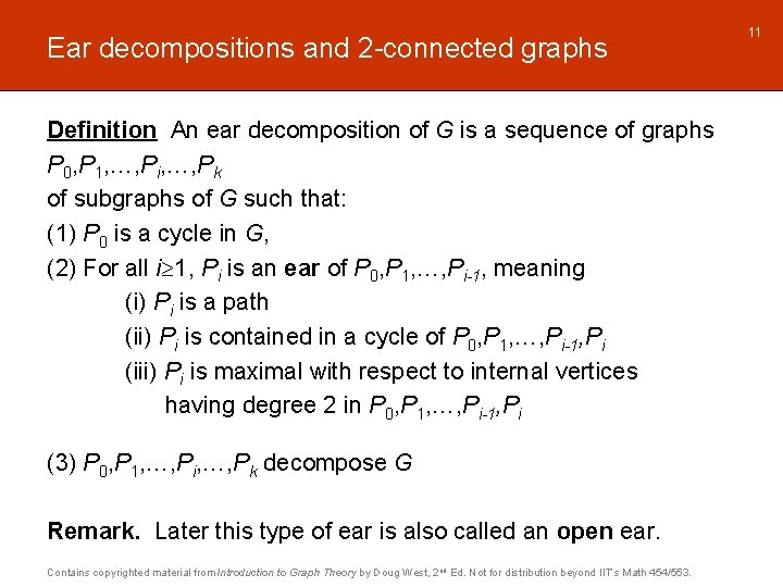
Ear decompositions and 2 -connected graphs Definition An ear decomposition of G is a sequence of graphs P 0, P 1, …, Pi, …, Pk of subgraphs of G such that: (1) P 0 is a cycle in G, (2) For all i 1, Pi is an ear of P 0, P 1, …, Pi-1, meaning (i) Pi is a path (ii) Pi is contained in a cycle of P 0, P 1, …, Pi-1, Pi (iii) Pi is maximal with respect to internal vertices having degree 2 in P 0, P 1, …, Pi-1, Pi (3) P 0, P 1, …, Pi, …, Pk decompose G Remark. Later this type of ear is also called an open ear. Contains copyrighted material from Introduction to Graph Theory by Doug West, 2 nd Ed. Not for distribution beyond IIT’s Math 454/553. 11

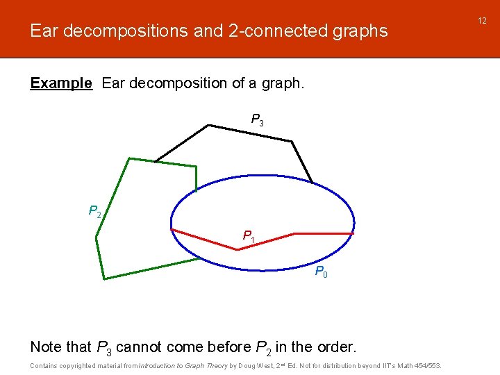
Ear decompositions and 2 -connected graphs Example Ear decomposition of a graph. P 3 P 2 P 1 P 0 Note that P 3 cannot come before P 2 in the order. Contains copyrighted material from Introduction to Graph Theory by Doug West, 2 nd Ed. Not for distribution beyond IIT’s Math 454/553. 12

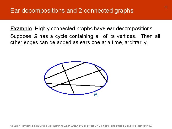
Ear decompositions and 2 -connected graphs Example Highly connected graphs have ear decompositions. Suppose G has a cycle containing all of its vertices. Then all other edges can be added as ears one at a time, arbitrarily. P 0 Contains copyrighted material from Introduction to Graph Theory by Doug West, 2 nd Ed. Not for distribution beyond IIT’s Math 454/553. 13

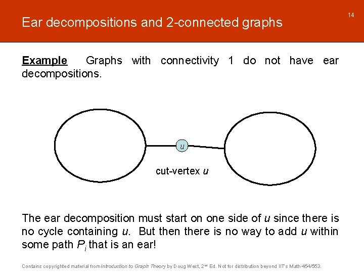
Ear decompositions and 2 -connected graphs Example Graphs with connectivity 1 do not have ear decompositions. u cut-vertex u The ear decomposition must start on one side of u since there is no cycle containing u. But then there is no way to add u within some path Pi that is an ear! Contains copyrighted material from Introduction to Graph Theory by Doug West, 2 nd Ed. Not for distribution beyond IIT’s Math 454/553. 14

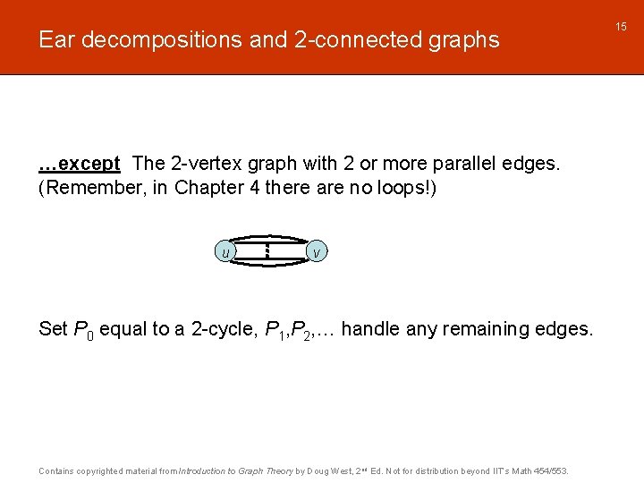
Ear decompositions and 2 -connected graphs …except The 2 -vertex graph with 2 or more parallel edges. (Remember, in Chapter 4 there are no loops!) u v Set P 0 equal to a 2 -cycle, P 1, P 2, … handle any remaining edges. Contains copyrighted material from Introduction to Graph Theory by Doug West, 2 nd Ed. Not for distribution beyond IIT’s Math 454/553. 15

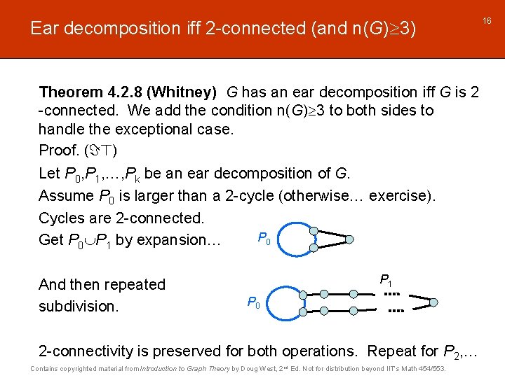
Ear decomposition iff 2 -connected (and n(G) 3) Theorem 4. 2. 8 (Whitney) G has an ear decomposition iff G is 2 -connected. We add the condition n(G) 3 to both sides to handle the exceptional case. Proof. (=>) Let P 0, P 1, …, Pk be an ear decomposition of G. Assume P 0 is larger than a 2 -cycle (otherwise… exercise). Cycles are 2 -connected. P 0 Get P 0 P 1 by expansion… And then repeated subdivision. P 1 P 0 2 -connectivity is preserved for both operations. Repeat for P 2, … Contains copyrighted material from Introduction to Graph Theory by Doug West, 2 nd Ed. Not for distribution beyond IIT’s Math 454/553. 16

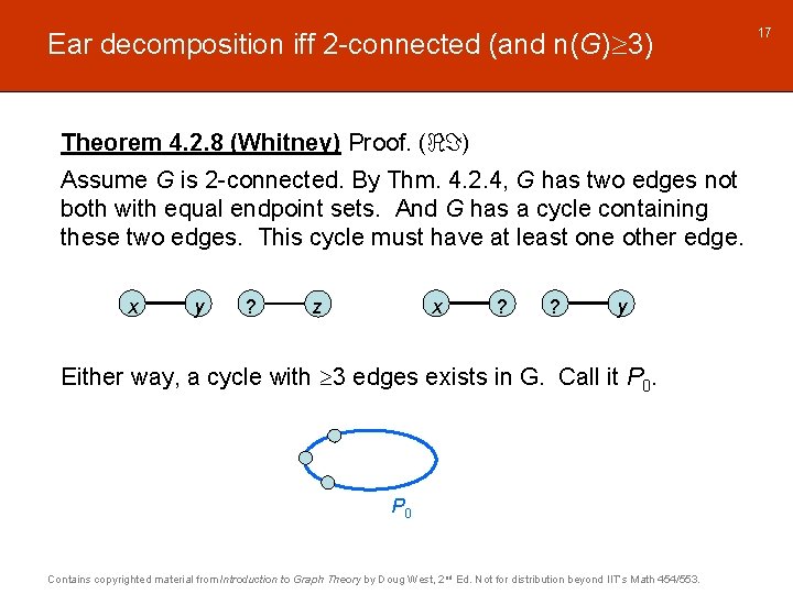
Ear decomposition iff 2 -connected (and n(G) 3) Theorem 4. 2. 8 (Whitney) Proof. (<=) Assume G is 2 -connected. By Thm. 4. 2. 4, G has two edges not both with equal endpoint sets. And G has a cycle containing these two edges. This cycle must have at least one other edge. x y ? x z ? ? y Either way, a cycle with 3 edges exists in G. Call it P 0 Contains copyrighted material from Introduction to Graph Theory by Doug West, 2 nd Ed. Not for distribution beyond IIT’s Math 454/553. 17

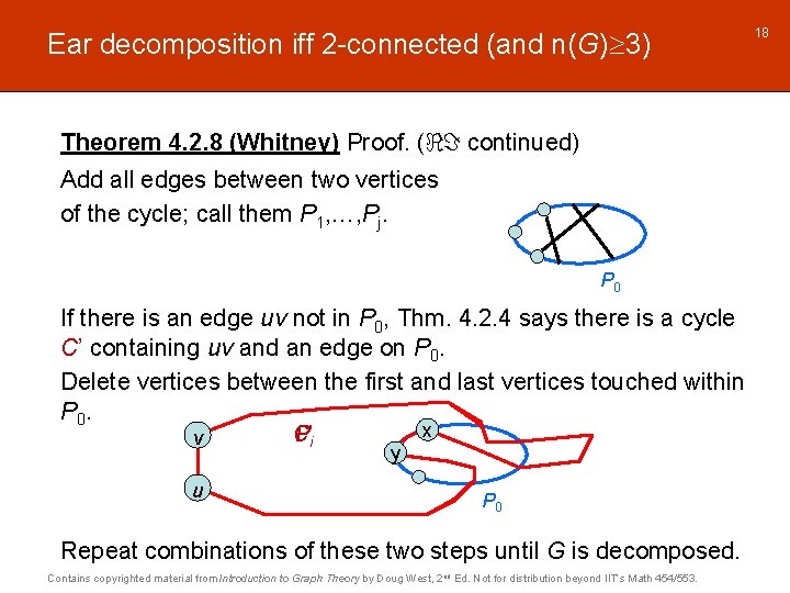
Ear decomposition iff 2 -connected (and n(G) 3) Theorem 4. 2. 8 (Whitney) Proof. (<= continued) Add all edges between two vertices of the cycle; call them P 1, …, Pj. P 0 If there is an edge uv not in P 0, Thm. 4. 2. 4 says there is a cycle C’ containing uv and an edge on P 0. Delete vertices between the first and last vertices touched within P 0. v u C’ Pi x y P 0 Repeat combinations of these two steps until G is decomposed. Contains copyrighted material from Introduction to Graph Theory by Doug West, 2 nd Ed. Not for distribution beyond IIT’s Math 454/553. 18

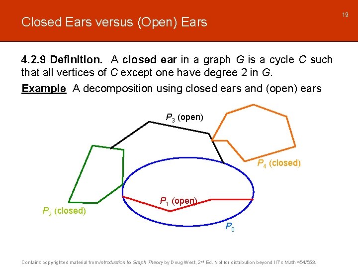
19 Closed Ears versus (Open) Ears 4. 2. 9 Definition. A closed ear in a graph G is a cycle C such that all vertices of C except one have degree 2 in G. Example A decomposition using closed ears and (open) ears P 3 (open) P 4 (closed) P 2 (closed) P 1 (open) P 0 Contains copyrighted material from Introduction to Graph Theory by Doug West, 2 nd Ed. Not for distribution beyond IIT’s Math 454/553.

Closed-Ear Decompositions and 2 -Edge-Connectivity A closed-ear decomposition of a graph G is a decomposition P 0, P 1, …, Pi, …, Pk such that P 0 is a cycle and Pi for i 1 is either an (open) ear or a closed ear in the union of P 0, P 1, …, Pi. 4. 2. 10 Theorem. A graph is 2 -connected iff it has a closed-ear decomposition, and every cycle in a 2 -edge-connected graph is the initial cycle in some such decomposition. The proof of Theorem 4. 2. 10 is quite similar to that of Theorem 4. 2. 8 (with 2 -connected iff ear decomposition). See p 164. (=>) Show 2 -edge-connectectedness is maintained on addition of each Pi. (<=) Find a cycle P 0 in G. Iteratively find add ears Pi containing an edge with one endpoint in the graph so far. Contains copyrighted material from Introduction to Graph Theory by Doug West, 2 nd Ed. Not for distribution beyond IIT’s Math 454/553. 20

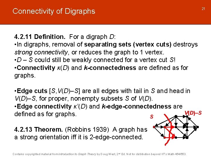
Connectivity of Digraphs 21 4. 2. 11 Definition. For a digraph D: • In digraphs, removal of separating sets (vertex cuts) destroys strong connectivity, or reduces the graph to 1 vertex. • D – S could still be weakly connected for a vertex cut S! • Connectivity κ(D) and k-connectedness are defined as for graphs. • Edge cuts [S, V(D)–S] are all edges with tail in S and head in V(D)–S, for proper, nonempty subsets S of V(D). • Edge connectivity κ’(D) and k-edge-connectedness are V(D)–S defined as for graphs. S 4. 2. 13 Theorem. (Robbins 1939) A graph has a strong orientation iff it is 2 -edge-connected. Contains copyrighted material from Introduction to Graph Theory by Doug West, 2 nd Ed. Not for distribution beyond IIT’s Math 454/553.

Local connectivity and Menger’s Theorem Local connectivity considers the number of alternative paths between a pair of vertices x, y, and the minimum size structure needed to be deleted to disconnect x from y. Global connectivity considers the minimum number of alternative paths between any pair of vertices, and the minimum size structure needed to be deleted to disconnect the graph. We have seen that (for n(G) 3) 2 -connectedness is equivalent to there existing 2 internally disjoint paths between any pair of vertices. We want to extend this idea: Locally: compare alternative x, y-paths versus minimum x, y-cuts Globally: find vertex pairs optimizing the local values Contains copyrighted material from Introduction to Graph Theory by Doug West, 2 nd Ed. Not for distribution beyond IIT’s Math 454/553. 22

Definitions for local connectivity 4. 2. 15 Definition. Let x, y V(G), S V(G)–{x, y}, F E(G), X, Y V(G) (1) S is an x, y-separator (also, x, y-cut) if G–S has no x, y-path (1’) κ(x, y) = minimum size of an x, y-separator (2) (x, y) = maximum # of pairwise internally disjoint x, y-paths (3) F is an x, y-disconnecting set if G-F has no x, y-path (3’) κ’(x, y) = minimum size of an x, y-disconnecting set (4) ’(x, y) = maximum # of pairwise edge-disjoint x, y-paths (5) An X, Y-path starts in X, ends in Y, otherwise avoids X Y Contains copyrighted material from Introduction to Graph Theory by Doug West, 2 nd Ed. Not for distribution beyond IIT’s Math 454/553. 23

24 Examples for local connectivity (1) 4. 2. 16 Example u x d w c z a b y v x, y-connectivity (x, y) 4 (4 int. disj. x, y-paths) κ(x, y) 4 (cut = ) u x d w c z a b y v w, z-connectivity (w, z) 3 (3 int. disj. w, z-paths) κ(w, z) 3 (cut = ) Contains copyrighted material from Introduction to Graph Theory by Doug West, 2 nd Ed. Not for distribution beyond IIT’s Math 454/553.

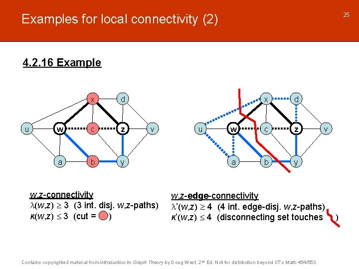
25 Examples for local connectivity (2) 4. 2. 16 Example u x d w c z a b y v w, z-connectivity (w, z) 3 (3 int. disj. w, z-paths) κ(w, z) 3 (cut = ) u x d w c z a b y v w, z-edge-connectivity ’(w, z) 4 (4 int. edge-disj. w, z-paths) κ’(w, z) 4 (disconnecting set touches Contains copyrighted material from Introduction to Graph Theory by Doug West, 2 nd Ed. Not for distribution beyond IIT’s Math 454/553. )

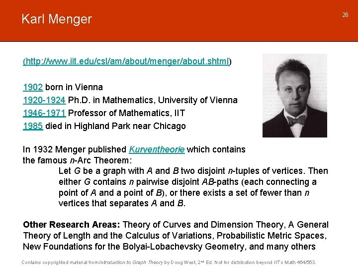
Karl Menger (http: //www. iit. edu/csl/am/about/menger/about. shtml) 1902 born in Vienna 1920 -1924 Ph. D. in Mathematics, University of Vienna 1946 -1971 Professor of Mathematics, IIT 1985 died in Highland Park near Chicago In 1932 Menger published Kurventheorie which contains the famous n-Arc Theorem: Let G be a graph with A and B two disjoint n-tuples of vertices. Then either G contains n pairwise disjoint AB-paths (each connecting a point of A and a point of B), or there exists a set of fewer than n vertices that separates A and B. Other Research Areas: Theory of Curves and Dimension Theory, A General Theory of Length and the Calculus of Variations, Probabilistic Metric Spaces, New Foundations for the Bolyai-Lobachevsky Geometry, and many others Contains copyrighted material from Introduction to Graph Theory by Doug West, 2 nd Ed. Not for distribution beyond IIT’s Math 454/553. 26

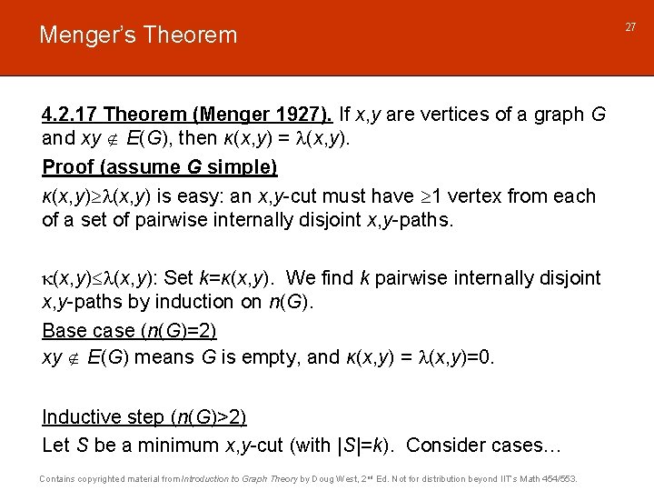
Menger’s Theorem 4. 2. 17 Theorem (Menger 1927). If x, y are vertices of a graph G and xy E(G), then κ(x, y) = (x, y). Proof (assume G simple) κ(x, y) is easy: an x, y-cut must have 1 vertex from each of a set of pairwise internally disjoint x, y-paths. (x, y): Set k=κ(x, y). We find k pairwise internally disjoint x, y-paths by induction on n(G). Base case (n(G)=2) xy E(G) means G is empty, and κ(x, y) = (x, y)=0. Inductive step (n(G)>2) Let S be a minimum x, y-cut (with |S|=k). Consider cases… Contains copyrighted material from Introduction to Graph Theory by Doug West, 2 nd Ed. Not for distribution beyond IIT’s Math 454/553. 27

28 Menger’s Theorem (2) Structure of G determines cases. Fact S does not properly contain N(x) or N(y). N(x) and N(y) are themselves x, y-cuts. Case 1 Exists S with S N(x) N(y). Define V 1=vertices of all x, S-paths V 2=vertices of all S, y-paths Properties of V 1, V 2: S = V 1 V 2 V 1 (N(y)-S) = V 2 (N(x)-S) = N(x) x S N(y) y G N(x) x S V 1 G Contains copyrighted material from Introduction to Graph Theory by Doug West, 2 nd Ed. Not for distribution beyond IIT’s Math 454/553. V 2

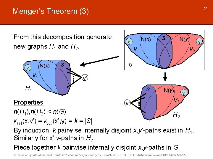
29 Menger’s Theorem (3) From this decomposition generate new graphs H 1 and H 2. x S G N(x) x V 1 H 1 N(x) S N(y) V 1 V 2 y’ S N(y) y V 2 Properties x’ n(H 1), n(H 2) < n(G) H 2 κH 1(x, y’) = κH 2(x’, y) = k = |S| By induction, k pairwise internally disjoint x, y’-paths exist in H 1. Similarly for x’, y-paths in H 2. Piece together k pairwise internally disjoint x, y-paths in G. Contains copyrighted material from Introduction to Graph Theory by Doug West, 2 nd Ed. Not for distribution beyond IIT’s Math 454/553. y

30 Menger’s Theorem (4) Case 2 All minimum x, y-cuts S satisfy S N(x) N(y). x N(x) N(y) y S G Case 2 A There exists some vertex v {x} N(x) N(y) {y}. Then v is in no minimum x, y-cut, and κ(G–v)=k. Induct on G-v to find κG-v(x, y) = k. Case 2 B There exists some vertex u N(x) N(y). Then u must be in every minimum x, y-cut in order to separate x from y. Therefore κ (G-u)=k-1. Induct on G-u to find G-u(x, y) = G-u(x, y)=k-1. Observe that the path x, u, y exists in G but not in G-u. Contains copyrighted material from Introduction to Graph Theory by Doug West, 2 nd Ed. Not for distribution beyond IIT’s Math 454/553.

31 Menger’s Theorem (5) N(x) N(y) x ge s G ed Case 2 C All minimum x, y-cuts S satisfy S N(x) N(y), and N(x), N(y) partition V(G)–{x, y}. y The set of x, y-paths are in natural bijection with the set of edges between N(x) and N(y). Therefore S is a vertex cover of G[N(x) N(y)] (bipartite). König-Egerváry gives a matching of size |S|=k. The matching edges correspond to pairwise internally disjoint x, y -paths, and so κ(x, y) = (x, y)=k. Contains copyrighted material from Introduction to Graph Theory by Doug West, 2 nd Ed. Not for distribution beyond IIT’s Math 454/553.

Menger’s Theorem 4. 2. 17 Theorem (Menger 1927). If x, y are vertices of a graph G and xy E(G), then κ(x, y) = (x, y). Proof (assume G simple) κ(x, y) is easy: an x, y-cut must have 1 vertex from each of a set of pairwise internally disjoint x, y-paths. (x, y): Set k=κ(x, y). We find k pairwise internally disjoint x, y-paths by induction on n(G). Base case (n(G)=2) xy E(G) means G is empty, and κ(x, y) = (x, y)=0. Inductive step (n(G)>2) Let S be a minimum x, y-cut (with |S|=k). Consider cases… Contains copyrighted material from Introduction to Graph Theory by Doug West, 2 nd Ed. Not for distribution beyond IIT’s Math 454/553. 32