Graph Mining in Social Network Analysis Professor Veljko

Graph Mining in Social Network Analysis Professor: Veljko Milutinović 1/17 Student: Dušan Ristić

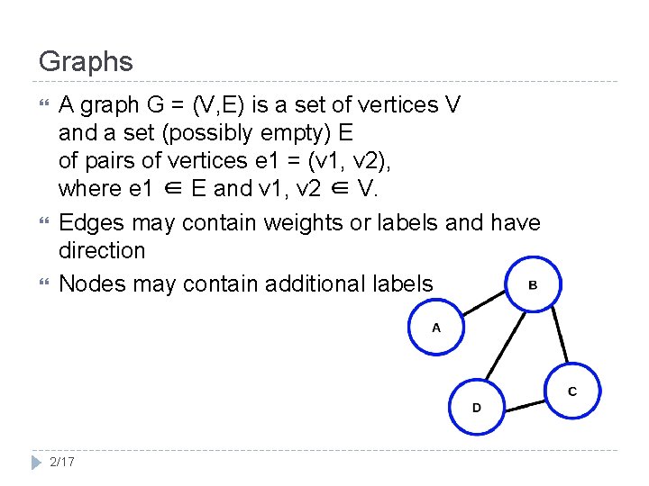
Graphs A graph G = (V, E) is a set of vertices V and a set (possibly empty) E of pairs of vertices e 1 = (v 1, v 2), where e 1 ∈ E and v 1, v 2 ∈ V. Edges may contain weights or labels and have direction Nodes may contain additional labels 2/17

Motivation Many domains produce data that can be intuitively represented by graphs. We would like to discover interesting facts and information about these graphs. Real world graph datasets are too large for humans to make any sense of. We would like to discover patterns that have structural information present. 3/17

Application Domains Web structure graphs Social networks Protein interaction networks Chemical compound Program Flow Transportation networks 4/17

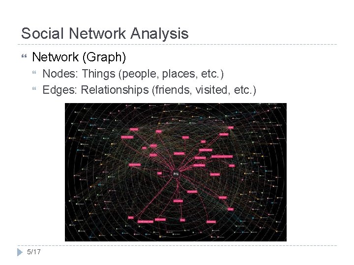
Social Network Analysis Network (Graph) 5/17 Nodes: Things (people, places, etc. ) Edges: Relationships (friends, visited, etc. )

Existing solutions Existing graph pattern mining algorithms: FSG g. Span Problems: 6/17 Fuzzy patterns Too many frequent subgraphs generated for large graphs

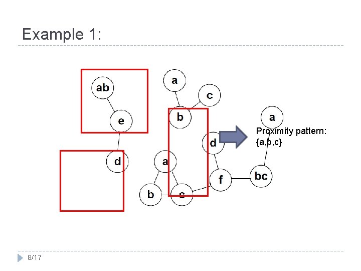
Proximity Pattern Overcomes the above two issues Subset of frequently repeating labels in tightly connected subgraphs 7/17

Example 1: Proximity pattern: {a, b, c} 8/17

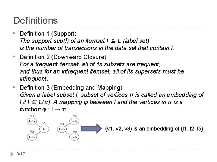
Definitions Definition 1 (Support) The support sup(I) of an itemset I ⊆ L (label set) is the number of transactions in the data set that contain I. Definition 2 (Downward Closure) For a frequent itemset, all of its subsets are frequent; and thus for an infrequent itemset, all of its supersets must be infrequent. Definition 3 (Embedding and Mapping) Given a label subset I, subset of vertices π is called an embedding of I if I ⊆ L(π). A mapping φ between I and the vertices in π is a function φ : I → π {v 1, v 2, v 3} is an embedding of {l 1, l 2, l 5} 9/17

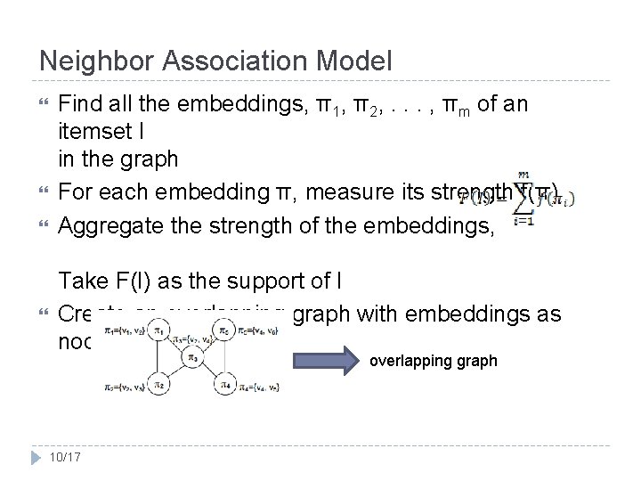
Neighbor Association Model Find all the embeddings, π1, π2, . . . , πm of an itemset I in the graph For each embedding π, measure its strength f(π) Aggregate the strength of the embeddings, Take F(I) as the support of I Create an overlapping graph with embeddings as nodes overlapping graph 10/17

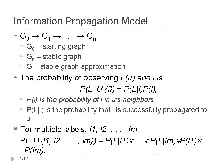
Information Propagation Model G 0 → G 1 →. . . → G n The probability of observing L(u) and l is: P(L ∪ {l}) = P(L|l)P(l), G 0 – starting graph Gn – stable graph G – stable graph approximation P(l) is the probability of l in u’s neighbors P(L|l) is the probability that l is successfully propagated to u For multiple labels, l 1, l 2, . . . , lm: P(L∪{l 1, l 2, . . . , lm}) = P(L|l 1)∗. . . ∗ P(L|lm)∗P(l 1)∗. . . P(lm). 11/17

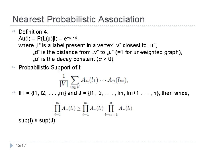
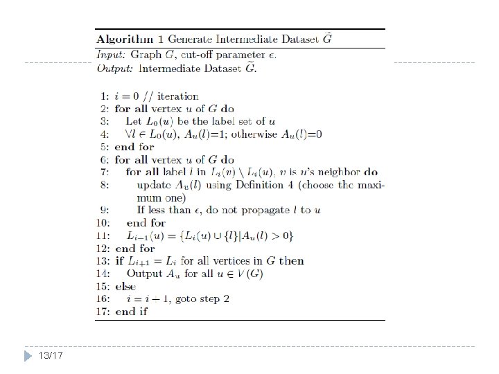
Nearest Probabilistic Association Definition 4. Au(l) = P(L(u)|l) = e−α・d, where „l‟ is a label present in a vertex „v‟ closest to „u‟, „d‟ is the distance from „v‟ to „u‟ (=1 for unweighted graph), „α‟ is the decay constant (α > 0) Probabilistic Support of I: If I = {l 1, l 2, . . . , m} and J = {l 1, l 2, . . . , lm+1. . . , n}, then since, sup(I) ≥ sup(J) 12/17

13/17

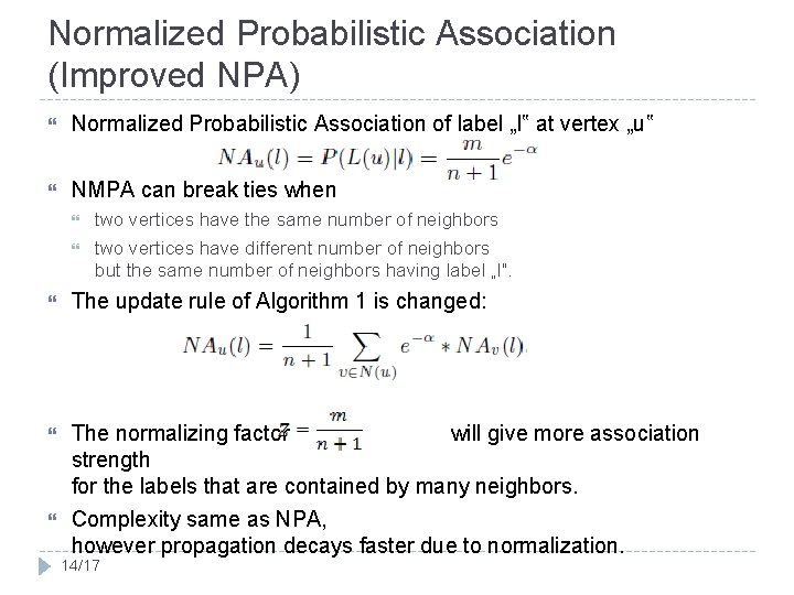
Normalized Probabilistic Association (Improved NPA) Normalized Probabilistic Association of label „l‟ at vertex „u‟ NMPA can break ties when two vertices have the same number of neighbors two vertices have different number of neighbors but the same number of neighbors having label „l‟. The update rule of Algorithm 1 is changed: The normalizing factor will give more association strength for the labels that are contained by many neighbors. Complexity same as NPA, however propagation decays faster due to normalization. 14/17

Conclusion With growth in popularity of social networks graph data mining will be more needed than ever Probabilistic itemset mining discovers new kind of patterns 15/17

Literature http: //cs. ucsb. edu/~xyan/papers/sigmod 10 association. pdf A. Khan, X. Yan, and K. -L. Wu. Towards proximity pattern mining in large graphs. In SIGMOD, 2010. C. C. Aggarwal, Y. Li, J. Wang. Frequent Pattern Mining with Uncertain Data. KDD 2009. Presentation on Frequent Pattern Growth (FPGrowth) Algorithm: An Introduction by Florian Verhein J. Han, J. Pei, Y. Yin. Mining frequent patterns without candidate generation. SIGMOD, 2000. 16/17

Questions? Dušan Ristić 3020/2014 E-mail: rd 143020 m@etf. rs 17/17