4 1 VQ Codeword Search 2 Vector Quantization

4. 1 VQ Codeword Search 2

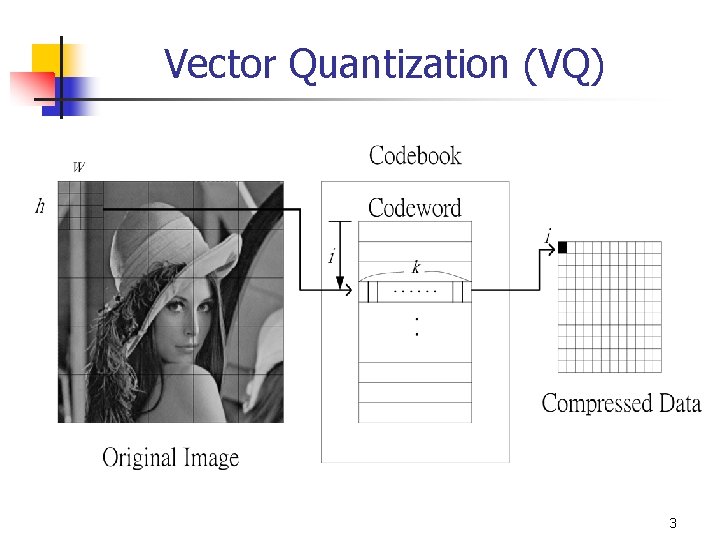
Vector Quantization (VQ) 3

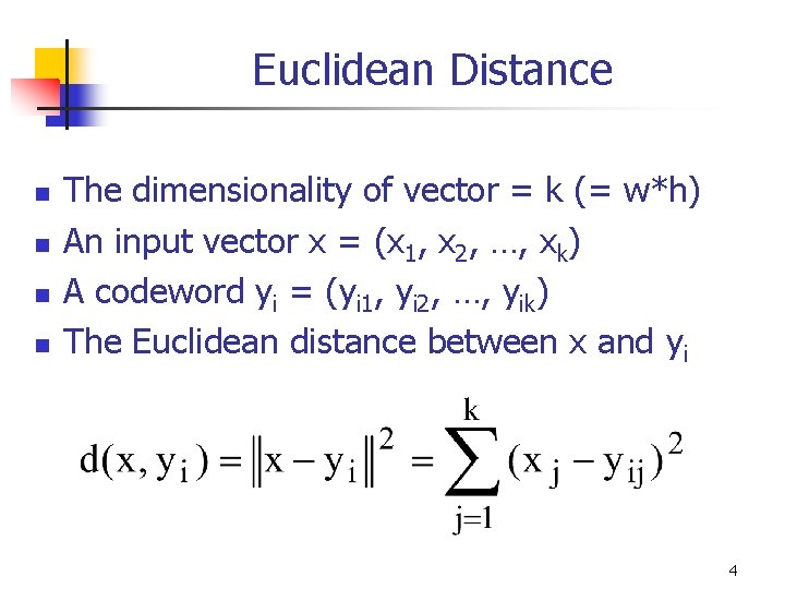
Euclidean Distance n n The dimensionality of vector = k (= w*h) An input vector x = (x 1, x 2, …, xk) A codeword yi = (yi 1, yi 2, …, yik) The Euclidean distance between x and yi 4

4. 2 PCA 5

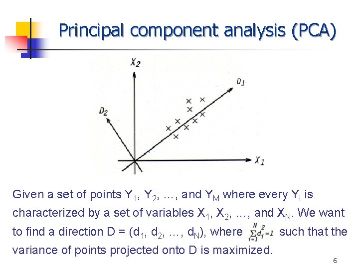
Principal component analysis (PCA) Given a set of points Y 1, Y 2, …, and YM where every Yi is characterized by a set of variables X 1, X 2, …, and XN. We want to find a direction D = (d 1, d 2, …, d. N), where variance of points projected onto D is maximized. such that the 6

Principal component analysis (PCA) n n D 1 = [0. 710 0. 703] D 2 = [-0. 703 0. 710] 7

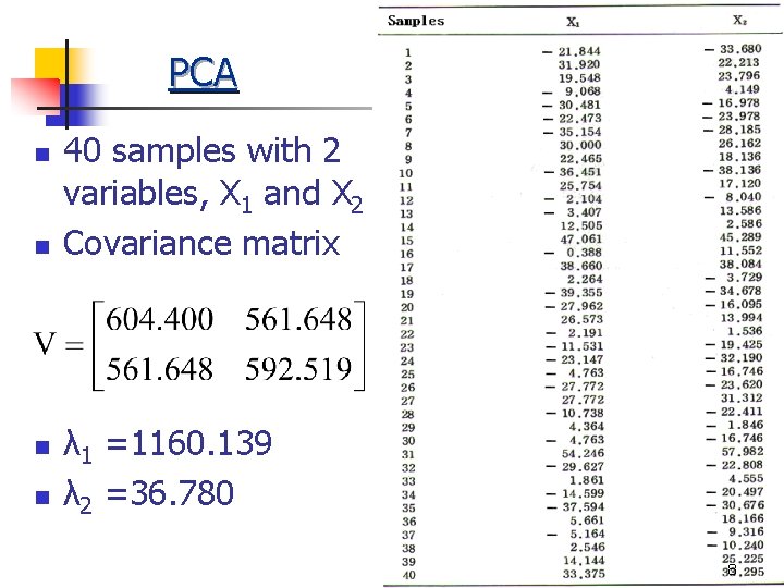
PCA n n 40 samples with 2 variables, X 1 and X 2 Covariance matrix λ 1 =1160. 139 λ 2 =36. 780 8

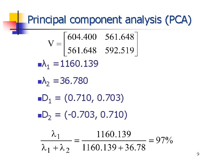
Principal component analysis (PCA) λ =1160. 139 n 1 λ =36. 780 n 2 n D 1 = (0. 710, 0. 703) n D 2 = (-0. 703, 0. 710) 9

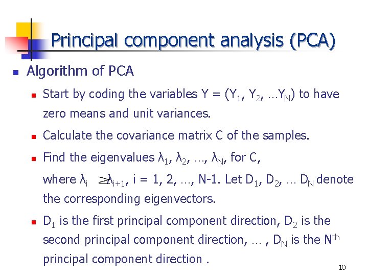
Principal component analysis (PCA) n Algorithm of PCA n Start by coding the variables Y = (Y 1, Y 2, …YN) to have zero means and unit variances. n Calculate the covariance matrix C of the samples. n Find the eigenvalues λ 1, λ 2, …, λN, for C, where λi λi+1, i = 1, 2, …, N-1. Let D 1, D 2, … DN denote the corresponding eigenvectors. n D 1 is the first principal component direction, D 2 is the second principal component direction, … , DN is the Nth principal component direction. 10

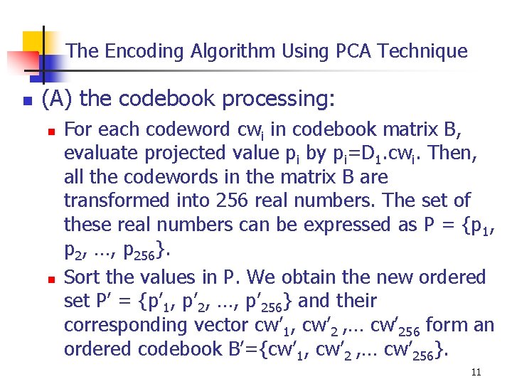
The Encoding Algorithm Using PCA Technique n (A) the codebook processing: n n For each codeword cwi in codebook matrix B, evaluate projected value pi by pi=D 1. cwi. Then, all the codewords in the matrix B are transformed into 256 real numbers. The set of these real numbers can be expressed as P = {p 1, p 2, …, p 256}. Sort the values in P. We obtain the new ordered set P’ = {p’ 1, p’ 2, …, p’ 256} and their corresponding vector cw’ 1, cw’ 2 , … cw’ 256 form an ordered codebook B’={cw’ 1, cw’ 2 , … cw’ 256}. 11

The Encoding Algorithm Using PCA Technique n (B) The Encoding Algorithm] n n For the input vector x, evaluate the projected value px by px = D 1. x. Search the set P’ for r values P’i’s which are the r closest ones to Px. Compute their distances from the set {cw’k, cw’k+1 , … cw’k+r-1} to find a vector cw’j such that (cw’j, x) has a minimum distortion. Here, let the searching range be r and assume that the corresponding codeword of P’j is cw’j. Store or transmit the index j of cw’j 12

The Encoding algorithm using PCA Codebook The covariance matrix 13

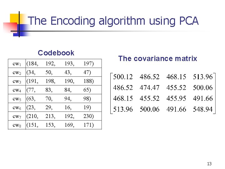
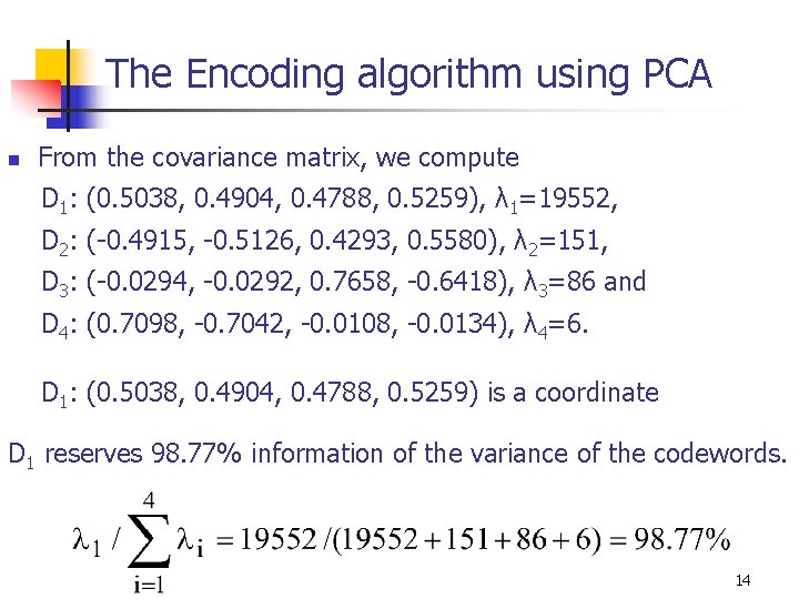
The Encoding algorithm using PCA n From the covariance matrix, we compute D 1: (0. 5038, 0. 4904, 0. 4788, 0. 5259), λ 1=19552, D 2: (-0. 4915, -0. 5126, 0. 4293, 0. 5580), λ 2=151, D 3: (-0. 0294, -0. 0292, 0. 7658, -0. 6418), λ 3=86 and D 4: (0. 7098, -0. 7042, -0. 0108, -0. 0134), λ 4=6. D 1: (0. 5038, 0. 4904, 0. 4788, 0. 5259) is a coordinate D 1 reserves 98. 77% information of the variance of the codewords. 14

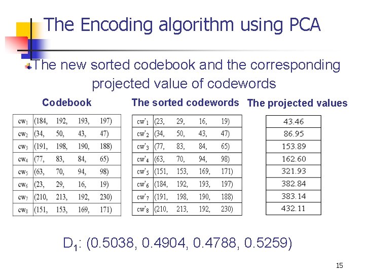
The Encoding algorithm using PCA The new sorted codebook and the corresponding projected value of codewords Codebook The sorted codewords The projected values D 1: (0. 5038, 0. 4904, 0. 4788, 0. 5259) 15

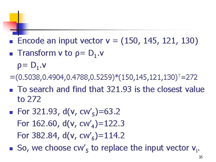
n n Encode an input vector v = (150, 145, 121, 130) Transform v to ρ= D 1. v =(0. 5038, 0. 4904, 0. 4788, 0. 5259)*(150, 145, 121, 130) T=272 n To search and find that 321. 93 is the closest value to 272 n For 321. 93, d(v, cw’ 5)=63. 2 For 162. 60, d(v, cw’ 4)=122. 3 For 382. 84, d(v, cw’ 6)=114. 2 n So, we choose cw’ 5 to replace the input vector vi. 16

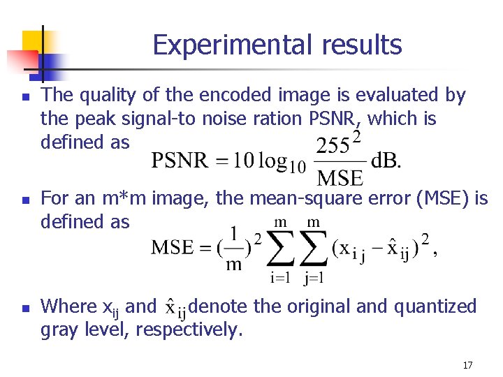
Experimental results n n n The quality of the encoded image is evaluated by the peak signal-to noise ration PSNR, which is defined as For an m*m image, the mean-square error (MSE) is defined as Where xij and denote the original and quantized gray level, respectively. 17

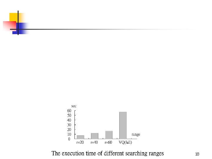
18

Look-up Table (LUT) The content of each pixel belongs to [0, m-1] 20

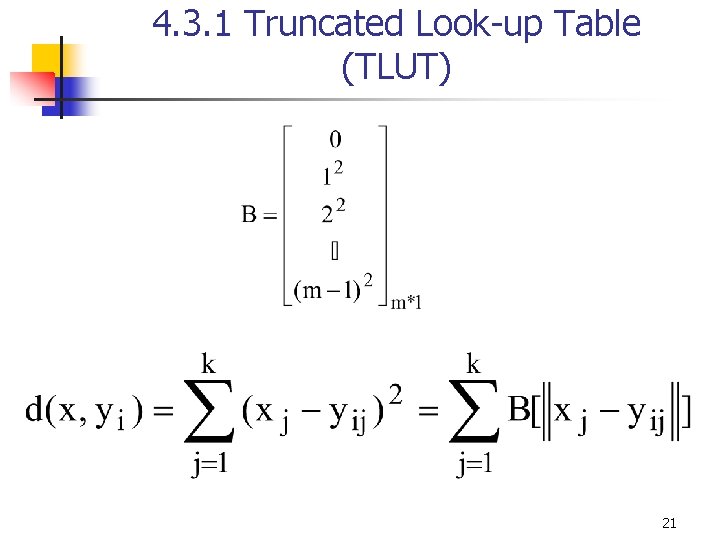
4. 3. 1 Truncated Look-up Table (TLUT) 21

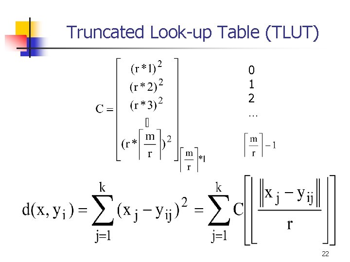
Truncated Look-up Table (TLUT) 0 1 2 … 22

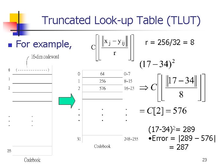
Truncated Look-up Table (TLUT) n For example, r = 256/32 = 8 (17 -34)2= 289 • Error = |289 – 576| = 287 23

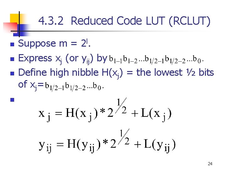
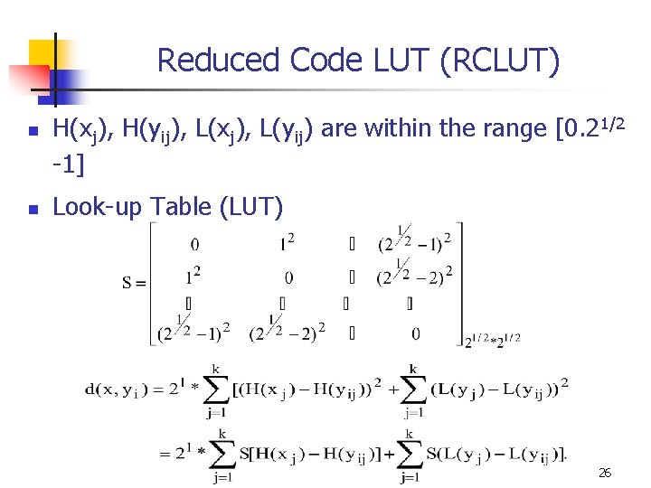
4. 3. 2 Reduced Code LUT (RCLUT) n n n Suppose m = 2 l. Express xj (or yij) by Define high nibble H(xj) = the lowest ½ bits of xj= n 24

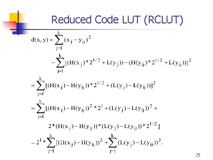
Reduced Code LUT (RCLUT) 25

Reduced Code LUT (RCLUT) n n H(xj), H(yij), L(xj), L(yij) are within the range [0. 21/2 -1] Look-up Table (LUT) 26

27

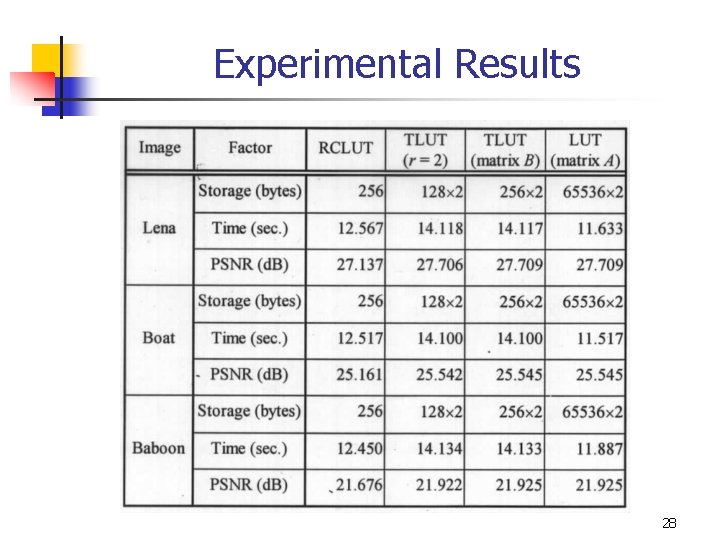
Experimental Results 28

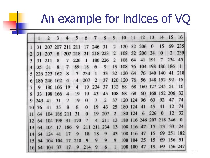
An example for indices of VQ 30

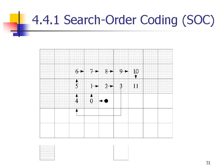
4. 4. 1 Search-Order Coding (SOC) 31

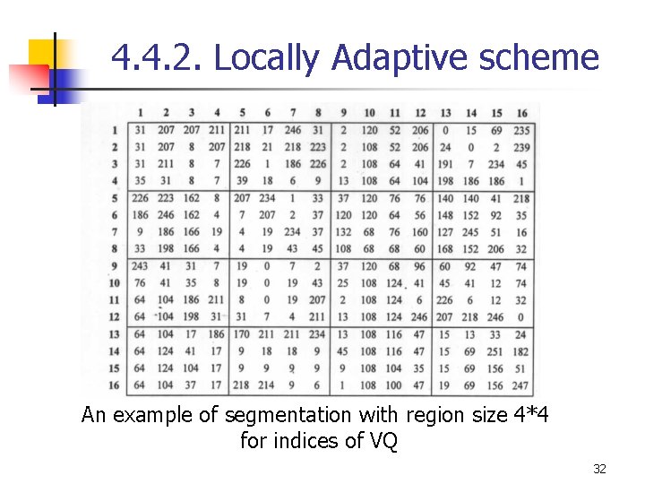
4. 4. 2. Locally Adaptive scheme An example of segmentation with region size 4*4 for indices of VQ 32

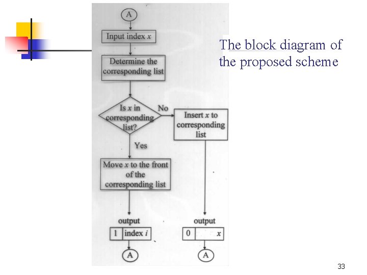
The block diagram of the proposed scheme 33

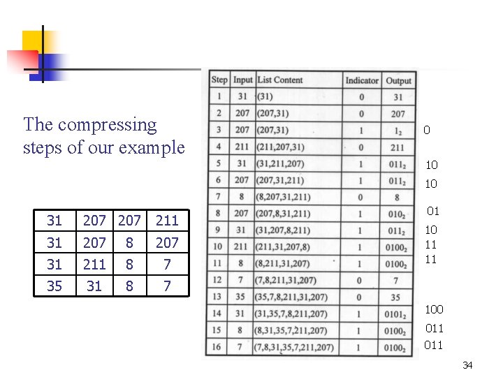
The compressing steps of our example 0 10 10 31 207 211 31 207 8 207 31 211 8 7 35 31 8 7 01 10 11 11 100 011 34

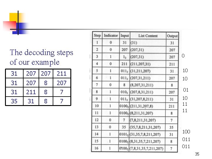
The decoding steps of our example 31 207 211 31 207 8 207 31 211 8 7 35 31 8 7 0 10 10 01 10 11 11 100 011 35

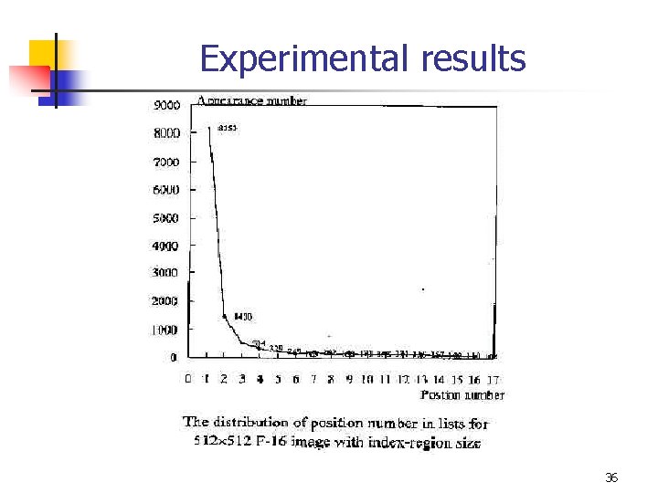
Experimental results 36

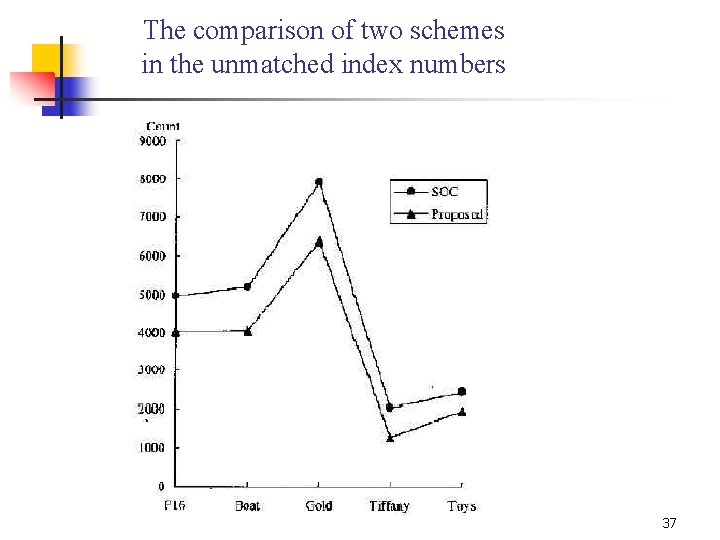
The comparison of two schemes in the unmatched index numbers 37

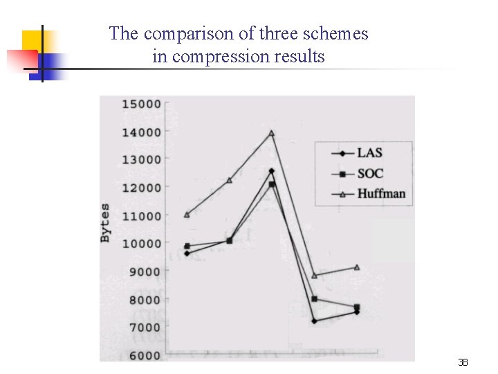
The comparison of three schemes in compression results 38

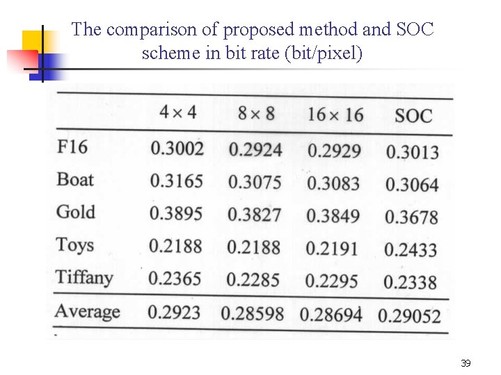
The comparison of proposed method and SOC scheme in bit rate (bit/pixel) 39

Discussions 40

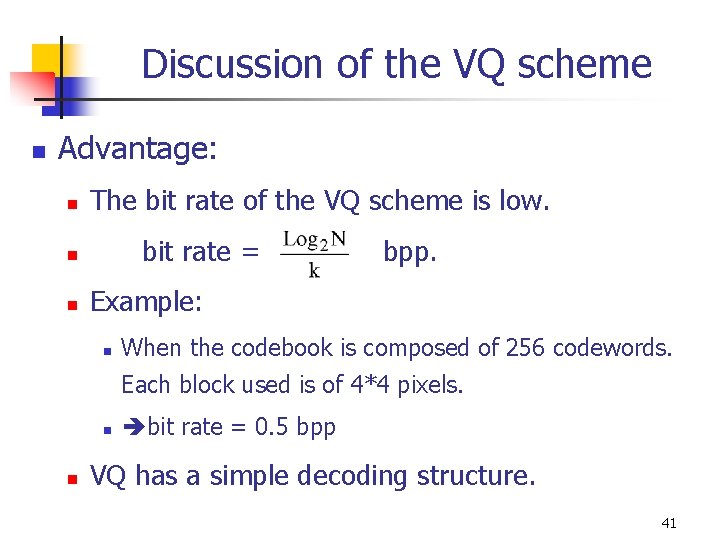
Discussion of the VQ scheme n Advantage: n The bit rate of the VQ scheme is low. bit rate = n n bpp. Example: n When the codebook is composed of 256 codewords. Each block used is of 4*4 pixels. n n bit rate = 0. 5 bpp VQ has a simple decoding structure. 41

Discussion of the VQ scheme n Disadvantage: n The reconstructed image quality highly depends on the codebook performance. n Therefore, how to design a representative codebook is an important issue of VQ scheme. n The VQ scheme requires a lot of computation cost in codebook generation process and VQ encoding process. 42