2013 Cengage Learning All Rights Reserved May not

© 2013 Cengage Learning. All Rights Reserved. May not be copied, scanned, or duplicated, in whole or in part, except for use as permitted in a license distributed with a certain product or service or otherwise on a password-protected website for classroom use.

Chapter 8: Multiple Regression for Time Series 8. 1 Graphical analysis and preliminary model development 8. 2 The multiple regression model 8. 3 Testing the overall model 8. 4 Testing individual coefficients 8. 5 Checking the assumptions 8. 6 Forecasting with multiple regression 8. 7 Principles 2 © 2013 Cengage Learning. All Rights Reserved. May not be copied, scanned, or duplicated, in whole or in part, except for use as permitted in a license distributed with a certain product or service or otherwise on a password-protected website for classroom use.

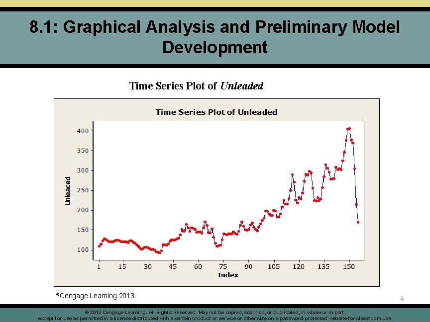
8. 1: Graphical Analysis and Preliminary Model Development • Suppose we are interested in the level of gas prices as a function of various explanatory variables. • Observe Gas Prices (=Yt) over n time periods, t = 1, 2, …, n Step 1: DDD, a time plot of Y against time Step 2: produce a scatter plot of Y against each explanatory variable Xj o For step 2, identify possible variables: § Personal Disposable Income § Unemployment § S&P 500 Index § Price of crude oil Q: What other variables would be of potential interest? 3 © 2013 Cengage Learning. All Rights Reserved. May not be copied, scanned, or duplicated, in whole or in part, except for use as permitted in a license distributed with a certain product or service or otherwise on a password-protected website for classroom use.

8. 1: Graphical Analysis and Preliminary Model Development Time Series Plot of Unleaded ©Cengage Learning 2013. © 2013 Cengage Learning. All Rights Reserved. May not be copied, scanned, or duplicated, in whole or in part, except for use as permitted in a license distributed with a certain product or service or otherwise on a password-protected website for classroom use. 4

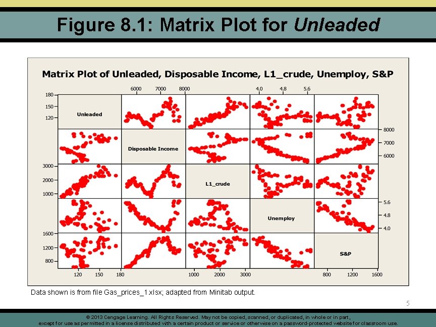
Figure 8. 1: Matrix Plot for Unleaded Data shown is from file Gas_prices_1. xlsx; adapted from Minitab output. 5 © 2013 Cengage Learning. All Rights Reserved. May not be copied, scanned, or duplicated, in whole or in part, except for use as permitted in a license distributed with a certain product or service or otherwise on a password-protected website for classroom use.

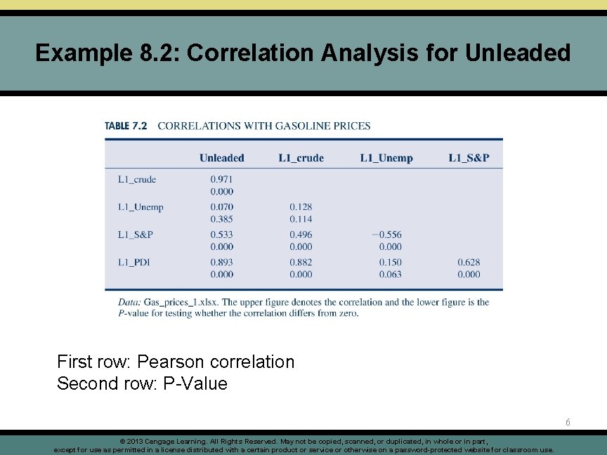
Example 8. 2: Correlation Analysis for Unleaded First row: Pearson correlation Second row: P-Value 6 © 2013 Cengage Learning. All Rights Reserved. May not be copied, scanned, or duplicated, in whole or in part, except for use as permitted in a license distributed with a certain product or service or otherwise on a password-protected website for classroom use.

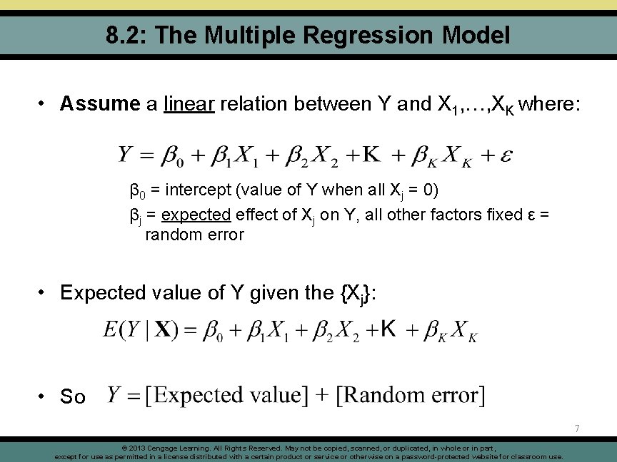
8. 2: The Multiple Regression Model • Assume a linear relation between Y and X 1, …, XK where: β 0 = intercept (value of Y when all Xj = 0) βj = expected effect of Xj on Y, all other factors fixed ε = random error • Expected value of Y given the {Xj}: • So 7 © 2013 Cengage Learning. All Rights Reserved. May not be copied, scanned, or duplicated, in whole or in part, except for use as permitted in a license distributed with a certain product or service or otherwise on a password-protected website for classroom use.

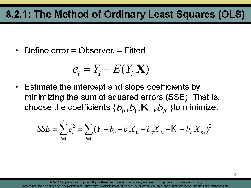
8. 2. 1: The Method of Ordinary Least Squares (OLS) • Define error = Observed – Fitted • Estimate the intercept and slope coefficients by minimizing the sum of squared errors (SSE). That is, choose the coefficients to minimize: 8 © 2013 Cengage Learning. All Rights Reserved. May not be copied, scanned, or duplicated, in whole or in part, except for use as permitted in a license distributed with a certain product or service or otherwise on a password-protected website for classroom use.

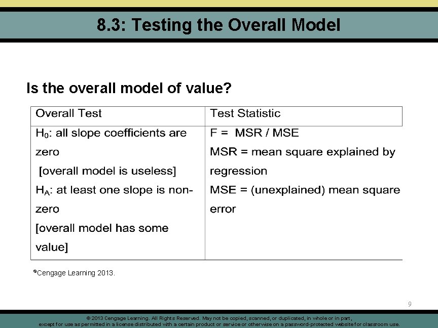
8. 3: Testing the Overall Model Is the overall model of value? ©Cengage Learning 2013. 9 © 2013 Cengage Learning. All Rights Reserved. May not be copied, scanned, or duplicated, in whole or in part, except for use as permitted in a license distributed with a certain product or service or otherwise on a password-protected website for classroom use.

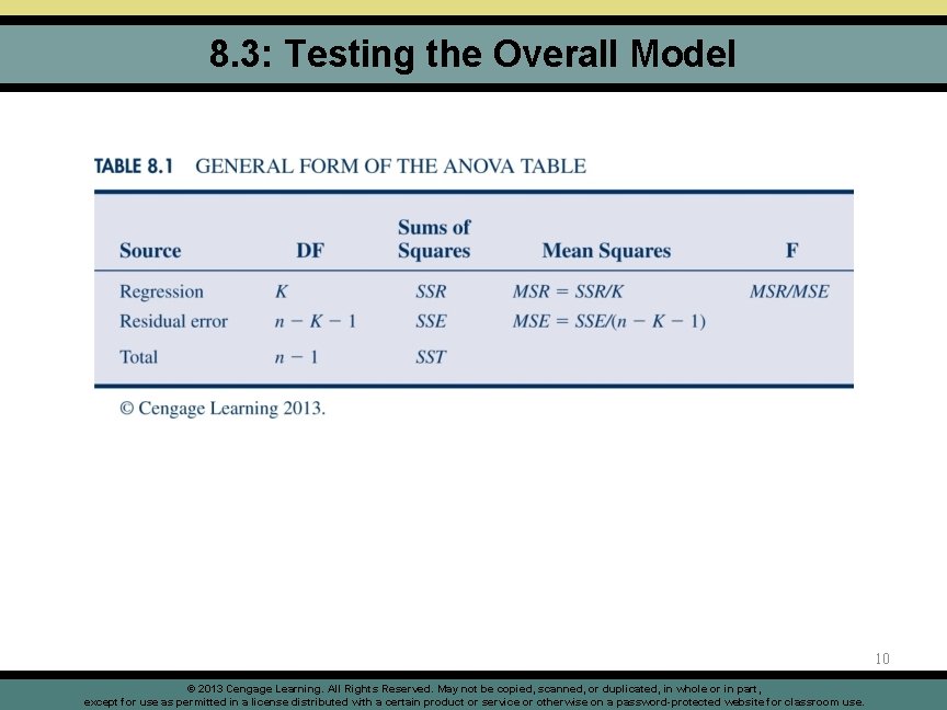
8. 3: Testing the Overall Model 10 © 2013 Cengage Learning. All Rights Reserved. May not be copied, scanned, or duplicated, in whole or in part, except for use as permitted in a license distributed with a certain product or service or otherwise on a password-protected website for classroom use.

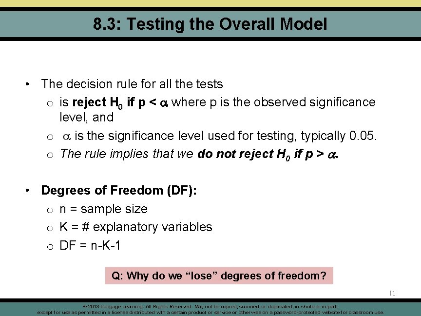
8. 3: Testing the Overall Model • The decision rule for all the tests o is reject H 0 if p < where p is the observed significance level, and o is the significance level used for testing, typically 0. 05. o The rule implies that we do not reject H 0 if p > . • Degrees of Freedom (DF): o n = sample size o K = # explanatory variables o DF = n-K-1 Q: Why do we “lose” degrees of freedom? 11 © 2013 Cengage Learning. All Rights Reserved. May not be copied, scanned, or duplicated, in whole or in part, except for use as permitted in a license distributed with a certain product or service or otherwise on a password-protected website for classroom use.

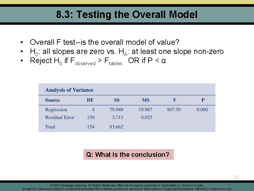
8. 3: Testing the Overall Model • Overall F test--is the overall model of value? • H 0: all slopes are zero vs. HA: at least one slope non-zero • Reject H 0 if Fobserved > Ftables OR if P < α Q: What is the conclusion? 12 © 2013 Cengage Learning. All Rights Reserved. May not be copied, scanned, or duplicated, in whole or in part, except for use as permitted in a license distributed with a certain product or service or otherwise on a password-protected website for classroom use.

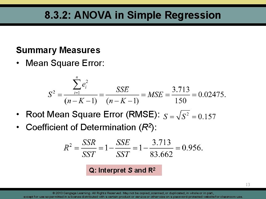
8. 3. 2: ANOVA in Simple Regression Summary Measures • Mean Square Error: • Root Mean Square Error (RMSE): • Coefficient of Determination (R 2): Q: Interpret S and R 2 13 © 2013 Cengage Learning. All Rights Reserved. May not be copied, scanned, or duplicated, in whole or in part, except for use as permitted in a license distributed with a certain product or service or otherwise on a password-protected website for classroom use.

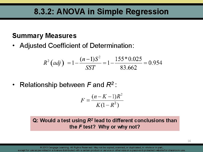
8. 3. 2: ANOVA in Simple Regression Summary Measures • Adjusted Coefficient of Determination: • Relationship between F and R 2 : Q: Would a test using R 2 lead to different conclusions than the F test? Why or why not? 14 © 2013 Cengage Learning. All Rights Reserved. May not be copied, scanned, or duplicated, in whole or in part, except for use as permitted in a license distributed with a certain product or service or otherwise on a password-protected website for classroom use.

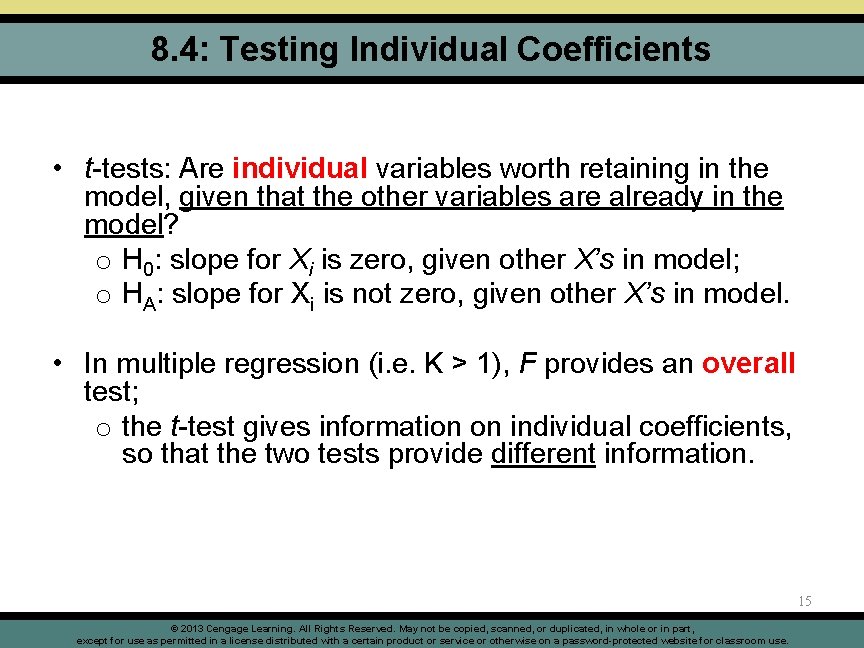
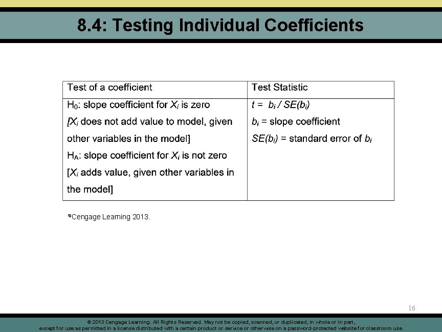
8. 4: Testing Individual Coefficients • t-tests: Are individual variables worth retaining in the model, given that the other variables are already in the model? o H 0: slope for Xi is zero, given other X’s in model; o HA: slope for Xi is not zero, given other X’s in model. • In multiple regression (i. e. K > 1), F provides an overall test; o the t-test gives information on individual coefficients, so that the two tests provide different information. 15 © 2013 Cengage Learning. All Rights Reserved. May not be copied, scanned, or duplicated, in whole or in part, except for use as permitted in a license distributed with a certain product or service or otherwise on a password-protected website for classroom use.

8. 4: Testing Individual Coefficients ©Cengage Learning 2013. 16 © 2013 Cengage Learning. All Rights Reserved. May not be copied, scanned, or duplicated, in whole or in part, except for use as permitted in a license distributed with a certain product or service or otherwise on a password-protected website for classroom use.

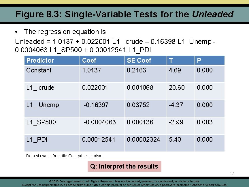
Figure 8. 3: Single-Variable Tests for the Unleaded • The regression equation is Unleaded = 1. 0137 + 0. 022001 L 1_ crude – 0. 16398 L 1_Unemp 0. 0004063 L 1_SP 500 + 0. 00012541 L 1_PDI Predictor Coef SE Coef T P Constant 1. 0137 0. 2163 4. 69 0. 000 L 1_ crude 0. 022001 0. 001068 20. 60 0. 000 L 1_ Unemp -0. 16397 0. 03752 -4. 37 0. 000 L 1_SP 500 -0. 0004063 0. 000136 -2. 99 0. 003 L 1_PDI 0. 00012541 0. 00002324 5. 40 0. 000 Data shown is from file Gas_prices_1. xlsx. Q: Interpret the results 17 © 2013 Cengage Learning. All Rights Reserved. May not be copied, scanned, or duplicated, in whole or in part, except for use as permitted in a license distributed with a certain product or service or otherwise on a password-protected website for classroom use.

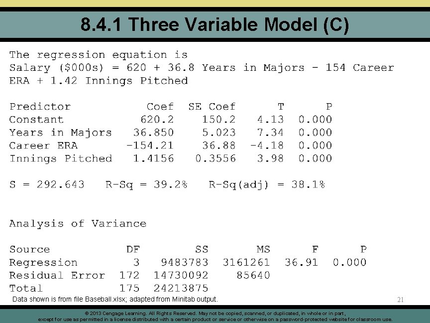
8. 4. 1: Case Study: Baseball Salaries • Examine the results for three and five variable models • What conclusions may be drawn? • How could the model be improved? 18 © 2013 Cengage Learning. All Rights Reserved. May not be copied, scanned, or duplicated, in whole or in part, except for use as permitted in a license distributed with a certain product or service or otherwise on a password-protected website for classroom use.

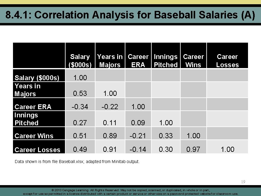
8. 4. 1: Correlation Analysis for Baseball Salaries (A) Salary Years in Career Innings Career ($000 s) Majors ERA Pitched Wins Salary ($000 s) Years in Majors 1. 00 0. 53 1. 00 Career ERA Innings Pitched -0. 34 -0. 22 1. 00 0. 27 0. 11 0. 09 1. 00 Career Wins 0. 51 0. 89 -0. 21 0. 33 1. 00 Career Losses 0. 49 0. 91 -0. 14 0. 30 0. 97 Career Losses 1. 00 Data shown is from file Baseball. xlsx; adapted from Minitab output. 19 © 2013 Cengage Learning. All Rights Reserved. May not be copied, scanned, or duplicated, in whole or in part, except for use as permitted in a license distributed with a certain product or service or otherwise on a password-protected website for classroom use.

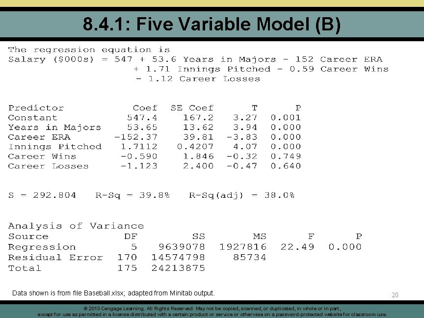
8. 4. 1: Five Variable Model (B) Data shown is from file Baseball. xlsx; adapted from Minitab output. © 2013 Cengage Learning. All Rights Reserved. May not be copied, scanned, or duplicated, in whole or in part, except for use as permitted in a license distributed with a certain product or service or otherwise on a password-protected website for classroom use. 20

8. 4. 1 Three Variable Model (C) Data shown is from file Baseball. xlsx; adapted from Minitab output. © 2013 Cengage Learning. All Rights Reserved. May not be copied, scanned, or duplicated, in whole or in part, except for use as permitted in a license distributed with a certain product or service or otherwise on a password-protected website for classroom use. 21

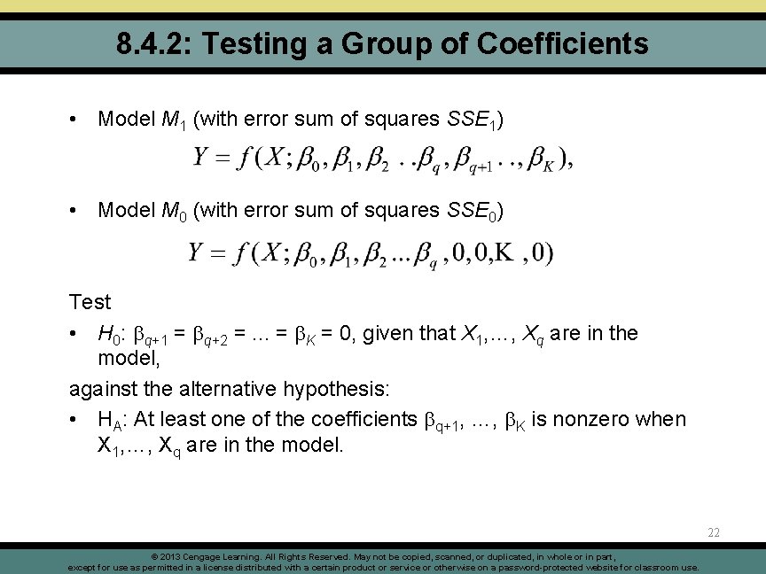
8. 4. 2: Testing a Group of Coefficients • Model M 1 (with error sum of squares SSE 1) • Model M 0 (with error sum of squares SSE 0) Test • H 0: q+1 = q+2 =. . . = K = 0, given that X 1, …, Xq are in the model, against the alternative hypothesis: • HA: At least one of the coefficients q+1, …, K is nonzero when X 1, …, Xq are in the model. 22 © 2013 Cengage Learning. All Rights Reserved. May not be copied, scanned, or duplicated, in whole or in part, except for use as permitted in a license distributed with a certain product or service or otherwise on a password-protected website for classroom use.

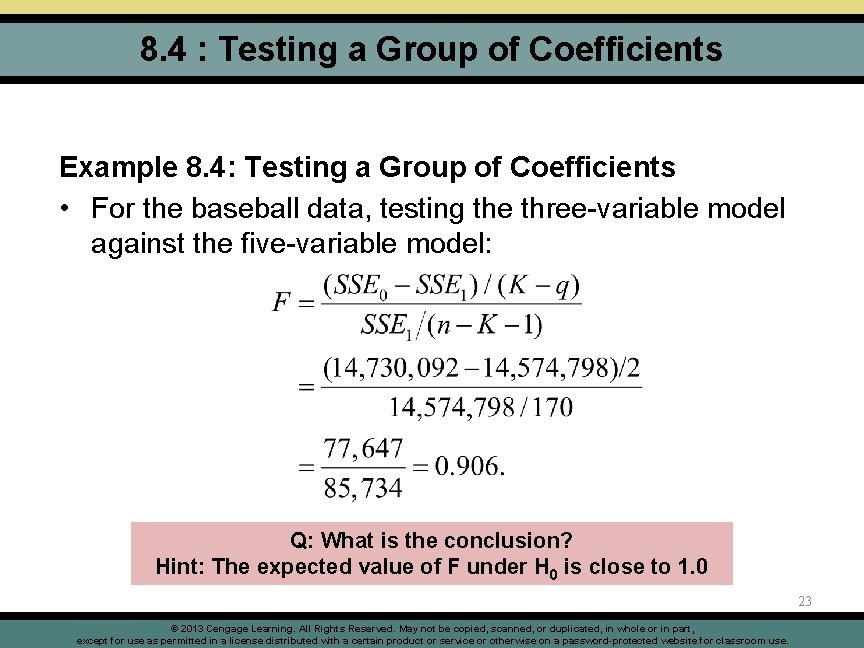
8. 4 : Testing a Group of Coefficients Example 8. 4: Testing a Group of Coefficients • For the baseball data, testing the three-variable model against the five-variable model: Q: What is the conclusion? Hint: The expected value of F under H 0 is close to 1. 0 23 © 2013 Cengage Learning. All Rights Reserved. May not be copied, scanned, or duplicated, in whole or in part, except for use as permitted in a license distributed with a certain product or service or otherwise on a password-protected website for classroom use.

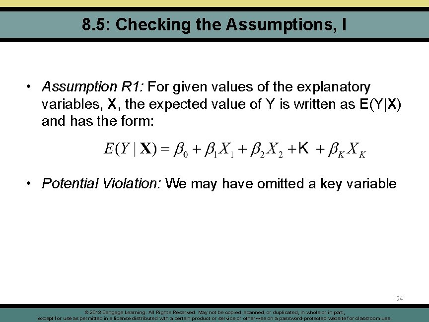
8. 5: Checking the Assumptions, I • Assumption R 1: For given values of the explanatory variables, X, the expected value of Y is written as E(Y|X) and has the form: • Potential Violation: We may have omitted a key variable 24 © 2013 Cengage Learning. All Rights Reserved. May not be copied, scanned, or duplicated, in whole or in part, except for use as permitted in a license distributed with a certain product or service or otherwise on a password-protected website for classroom use.

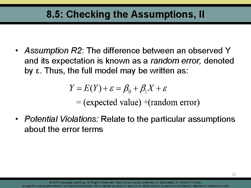
8. 5: Checking the Assumptions, II • Assumption R 2: The difference between an observed Y and its expectation is known as a random error, denoted by ε. Thus, the full model may be written as: • Potential Violations: Relate to the particular assumptions about the error terms 25 © 2013 Cengage Learning. All Rights Reserved. May not be copied, scanned, or duplicated, in whole or in part, except for use as permitted in a license distributed with a certain product or service or otherwise on a password-protected website for classroom use.

8. 5: Checking the Assumptions, III • Assumption R 3: The expected value of each error term is zero. That is there is no bias in the measurement process. • Potential Violation: Observations may contain bias. This assumption is not directly testable 26 © 2013 Cengage Learning. All Rights Reserved. May not be copied, scanned, or duplicated, in whole or in part, except for use as permitted in a license distributed with a certain product or service or otherwise on a password-protected website for classroom use.

8. 5: Checking the Assumptions, IV • Assumption R 4: The errors for different observations are uncorrelated with one another. When examining observations over time, this assumption corresponds to a lack of autocorrelation among the errors. • Potential Violation: The errors may be (auto)correlated. 27 © 2013 Cengage Learning. All Rights Reserved. May not be copied, scanned, or duplicated, in whole or in part, except for use as permitted in a license distributed with a certain product or service or otherwise on a password-protected website for classroom use.

8. 5: Checking the Assumptions, V • Assumption R 5: The variance of the errors is constant. That is, the error terms come from distributions with equal variances. When the assumption is satisfied the error process is homoscedastic. • Potential Violation: The variances are unequal; the error process is heteroscedastic. 28 © 2013 Cengage Learning. All Rights Reserved. May not be copied, scanned, or duplicated, in whole or in part, except for use as permitted in a license distributed with a certain product or service or otherwise on a password-protected website for classroom use.

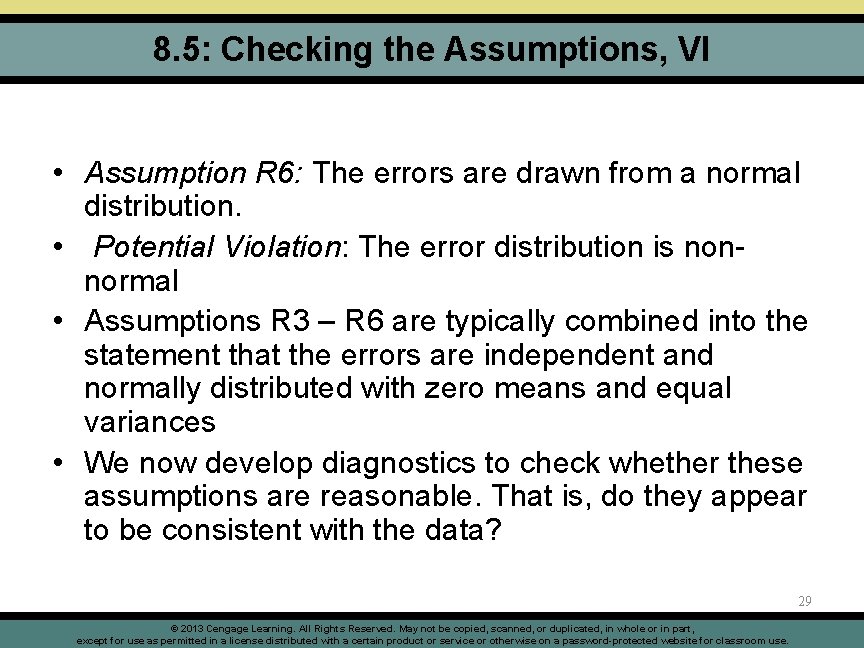
8. 5: Checking the Assumptions, VI • Assumption R 6: The errors are drawn from a normal distribution. • Potential Violation: The error distribution is nonnormal • Assumptions R 3 – R 6 are typically combined into the statement that the errors are independent and normally distributed with zero means and equal variances • We now develop diagnostics to check whether these assumptions are reasonable. That is, do they appear to be consistent with the data? 29 © 2013 Cengage Learning. All Rights Reserved. May not be copied, scanned, or duplicated, in whole or in part, except for use as permitted in a license distributed with a certain product or service or otherwise on a password-protected website for classroom use.

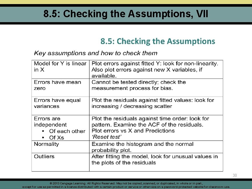
8. 5: Checking the Assumptions, VII 30 © 2013 Cengage Learning. All Rights Reserved. May not be copied, scanned, or duplicated, in whole or in part, except for use as permitted in a license distributed with a certain product or service or otherwise on a password-protected website for classroom use.

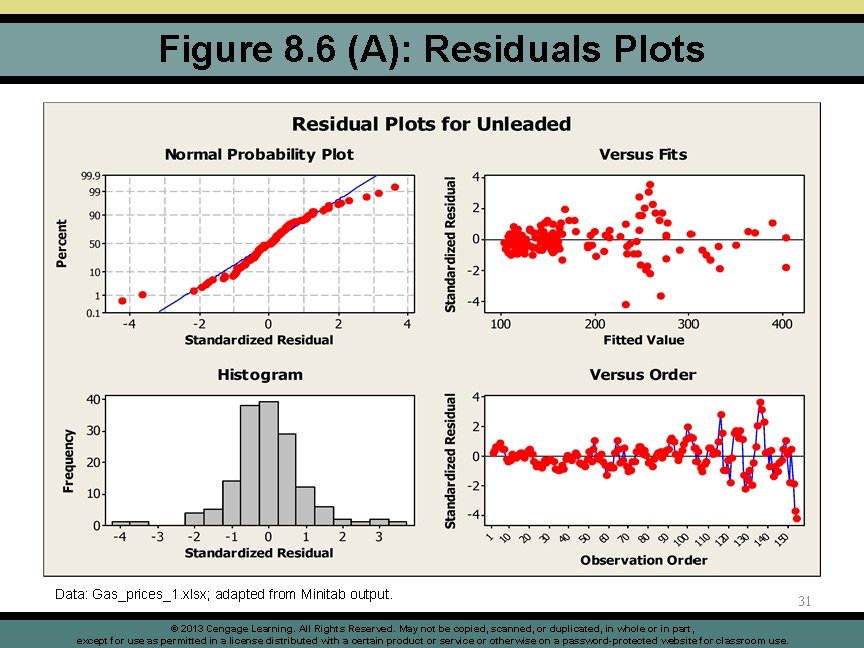
Figure 8. 6 (A): Residuals Plots Data: Gas_prices_1. xlsx; adapted from Minitab output. © 2013 Cengage Learning. All Rights Reserved. May not be copied, scanned, or duplicated, in whole or in part, except for use as permitted in a license distributed with a certain product or service or otherwise on a password-protected website for classroom use. 31

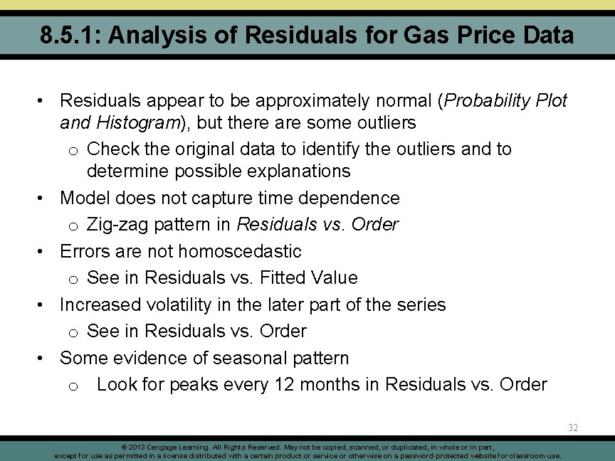
8. 5. 1: Analysis of Residuals for Gas Price Data • Residuals appear to be approximately normal (Probability Plot and Histogram), but there are some outliers o Check the original data to identify the outliers and to determine possible explanations • Model does not capture time dependence o Zig-zag pattern in Residuals vs. Order • Errors are not homoscedastic o See in Residuals vs. Fitted Value • Increased volatility in the later part of the series o See in Residuals vs. Order • Some evidence of seasonal pattern o Look for peaks every 12 months in Residuals vs. Order 32 © 2013 Cengage Learning. All Rights Reserved. May not be copied, scanned, or duplicated, in whole or in part, except for use as permitted in a license distributed with a certain product or service or otherwise on a password-protected website for classroom use.

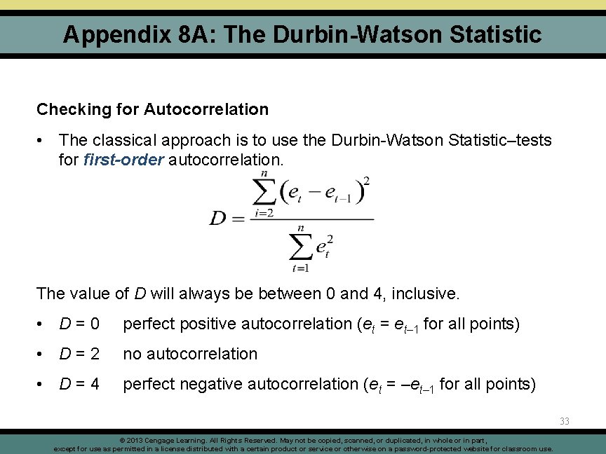
Appendix 8 A: The Durbin-Watson Statistic Checking for Autocorrelation • The classical approach is to use the Durbin-Watson Statistic–tests for first-order autocorrelation. The value of D will always be between 0 and 4, inclusive. • D=0 perfect positive autocorrelation (et = et– 1 for all points) • D=2 no autocorrelation • D=4 perfect negative autocorrelation (et = –et– 1 for all points) 33 © 2013 Cengage Learning. All Rights Reserved. May not be copied, scanned, or duplicated, in whole or in part, except for use as permitted in a license distributed with a certain product or service or otherwise on a password-protected website for classroom use.

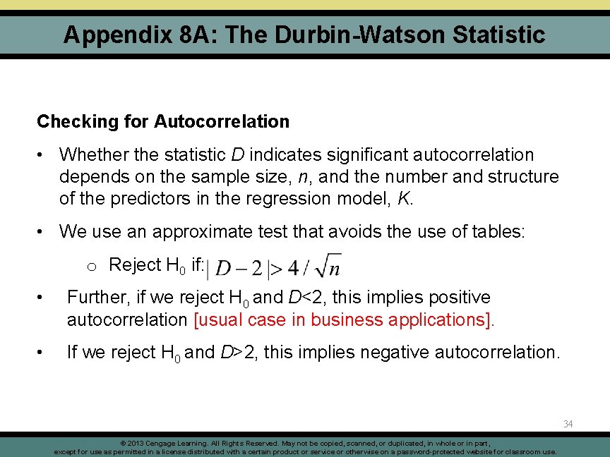
Appendix 8 A: The Durbin-Watson Statistic Checking for Autocorrelation • Whether the statistic D indicates significant autocorrelation depends on the sample size, n, and the number and structure of the predictors in the regression model, K. • We use an approximate test that avoids the use of tables: o Reject H 0 if: • Further, if we reject H 0 and D<2, this implies positive autocorrelation [usual case in business applications]. • If we reject H 0 and D>2, this implies negative autocorrelation. 34 © 2013 Cengage Learning. All Rights Reserved. May not be copied, scanned, or duplicated, in whole or in part, except for use as permitted in a license distributed with a certain product or service or otherwise on a password-protected website for classroom use.

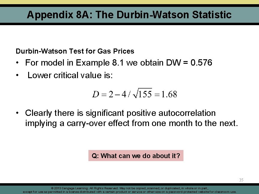
Appendix 8 A: The Durbin-Watson Statistic Durbin-Watson Test for Gas Prices • For model in Example 8. 1 we obtain DW = 0. 576 • Lower critical value is: • Clearly there is significant positive autocorrelation implying a carry-over effect from one month to the next. Q: What can we do about it? 35 © 2013 Cengage Learning. All Rights Reserved. May not be copied, scanned, or duplicated, in whole or in part, except for use as permitted in a license distributed with a certain product or service or otherwise on a password-protected website for classroom use.

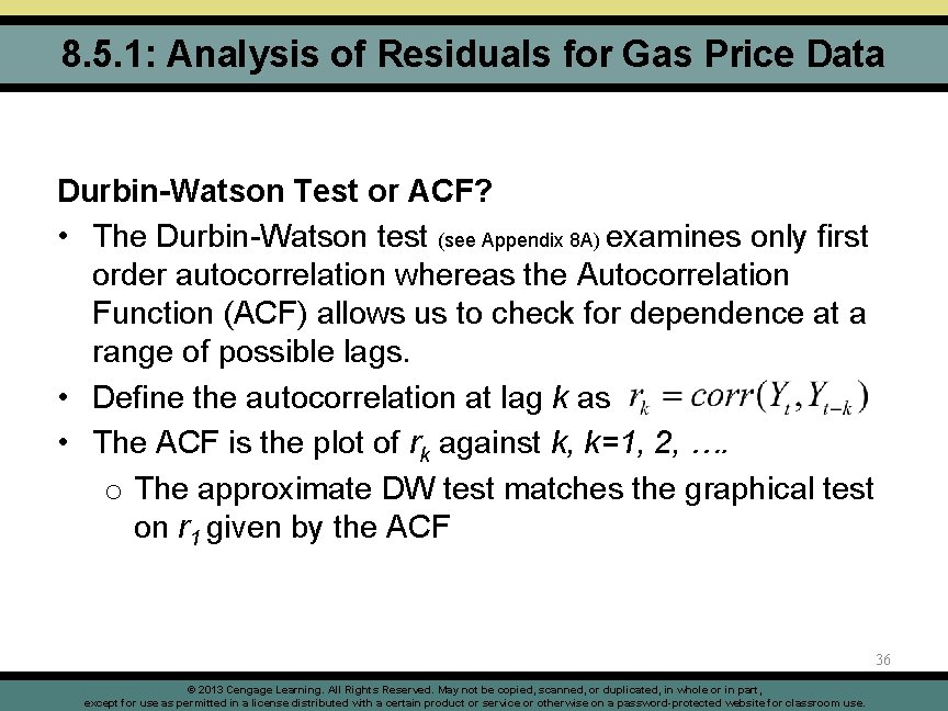
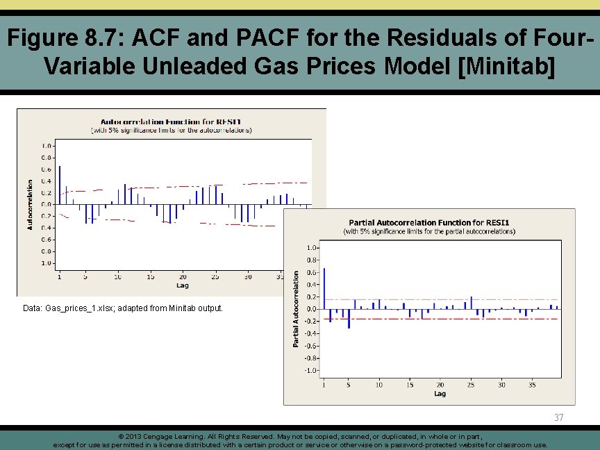
8. 5. 1: Analysis of Residuals for Gas Price Data Durbin-Watson Test or ACF? • The Durbin-Watson test (see Appendix 8 A) examines only first order autocorrelation whereas the Autocorrelation Function (ACF) allows us to check for dependence at a range of possible lags. • Define the autocorrelation at lag k as • The ACF is the plot of rk against k, k=1, 2, …. o The approximate DW test matches the graphical test on r 1 given by the ACF 36 © 2013 Cengage Learning. All Rights Reserved. May not be copied, scanned, or duplicated, in whole or in part, except for use as permitted in a license distributed with a certain product or service or otherwise on a password-protected website for classroom use.

Figure 8. 7: ACF and PACF for the Residuals of Four. Variable Unleaded Gas Prices Model [Minitab] Data: Gas_prices_1. xlsx; adapted from Minitab output. 37 © 2013 Cengage Learning. All Rights Reserved. May not be copied, scanned, or duplicated, in whole or in part, except for use as permitted in a license distributed with a certain product or service or otherwise on a password-protected website for classroom use.

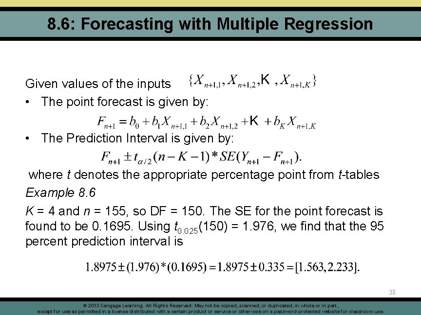
8. 6: Forecasting with Multiple Regression Given values of the inputs • The point forecast is given by: • The Prediction Interval is given by: where t denotes the appropriate percentage point from t-tables Example 8. 6 K = 4 and n = 155, so DF = 150. The SE for the point forecast is found to be 0. 1695. Using t 0. 025(150) = 1. 976, we find that the 95 percent prediction interval is 38 © 2013 Cengage Learning. All Rights Reserved. May not be copied, scanned, or duplicated, in whole or in part, except for use as permitted in a license distributed with a certain product or service or otherwise on a password-protected website for classroom use.

8. 7: Principles • Aim for a relatively simple model specification • Tailor the forecasting model to the horizon • Identify important causal variables on the basis of the underlying theory and earlier empirical studies. Identify suitable proxy variables when the variables of interest are not available in a timely fashion. • If the aim of the analysis is to provide pure forecasts o know the explanatory variables in advance o or be able to forecast them sufficiently well to justify their inclusion in the model. • Use the method of ordinary lest squares to estimate the parameters. • Update the estimates frequently. 39 © 2013 Cengage Learning. All Rights Reserved. May not be copied, scanned, or duplicated, in whole or in part, except for use as permitted in a license distributed with a certain product or service or otherwise on a password-protected website for classroom use.

Chapter 8: Take-Aways • Start the modeling process by careful consideration of available theory and previous empirical studies • Carry out a full preliminary analysis of the data to look for associations and for unusual observations • Test both the overall model and the individual components • Examine the validity of the underlying assumptions • Make sure that the model is “sensible” with respect to the signs and magnitudes of the slope coefficients • Use a hold-out sample to evaluate forecasting performance. 40 © 2013 Cengage Learning. All Rights Reserved. May not be copied, scanned, or duplicated, in whole or in part, except for use as permitted in a license distributed with a certain product or service or otherwise on a password-protected website for classroom use.