2013 Cengage Learning All Rights Reserved May not

© 2013 Cengage Learning. All Rights Reserved. May not be copied, scanned, or duplicated, in whole or in part, except for use as permitted in a license distributed with a certain product or service or otherwise on a password-protected website for classroom use.

Chapter 7: Simple Linear Regression for Forecasting 7. 1 Relationships Between Variables: Correlation and Causation 7. 2 Fitting a Regression Line by Ordinary Least Square (OLS) 7. 3 A Case Study on the Price of Gasoline 7. 4 How Good is the Fitted Line? 7. 5 The Statistical Framework for Regression 7. 6 Testing the Slope 7. 7 Forecasting by Using Simple Linear Regression 7. 8 Forecasting by Using Leading Indicators 2 © 2013 Cengage Learning. All Rights Reserved. May not be copied, scanned, or duplicated, in whole or in part, except for use as permitted in a license distributed with a certain product or service or otherwise on a password-protected website for classroom use.

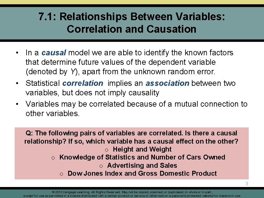
7. 1: Relationships Between Variables: Correlation and Causation • In a causal model we are able to identify the known factors that determine future values of the dependent variable (denoted by Y), apart from the unknown random error. • Statistical correlation implies an association between two variables, but does not imply causality • Variables may be correlated because of a mutual connection to other variables. Q: The following pairs of variables are correlated. Is there a causal relationship? If so, which variable has a causal effect on the other? o Height and Weight o Knowledge of Statistics and Number of Cars Owned o Advertising and Sales o Dow Jones Index and Gross Domestic Product 3 © 2013 Cengage Learning. All Rights Reserved. May not be copied, scanned, or duplicated, in whole or in part, except for use as permitted in a license distributed with a certain product or service or otherwise on a password-protected website for classroom use.

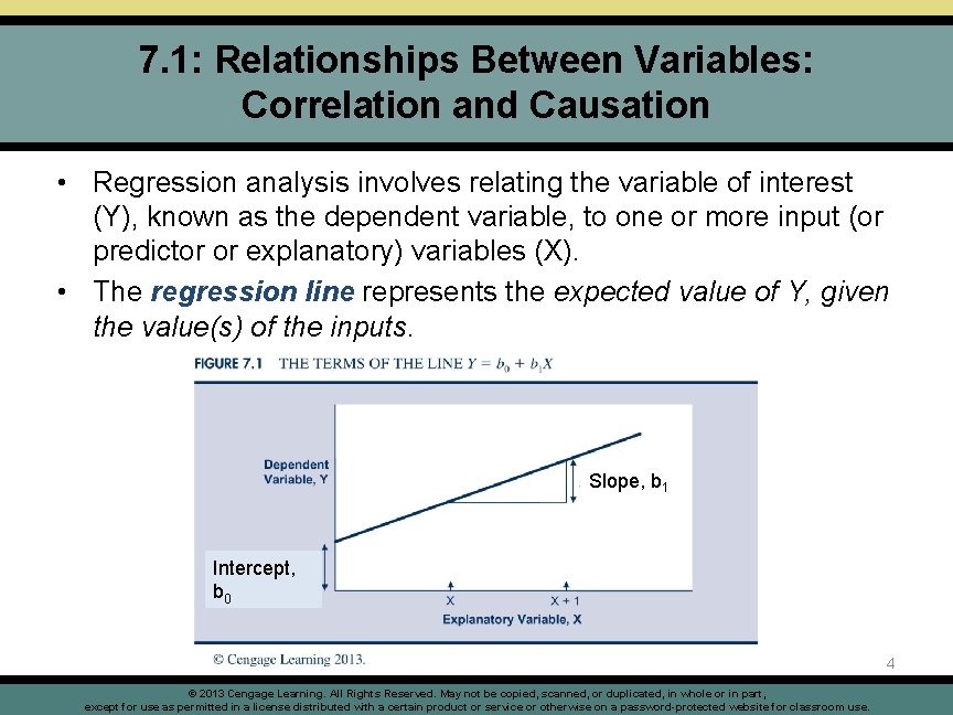
7. 1: Relationships Between Variables: Correlation and Causation • Regression analysis involves relating the variable of interest (Y), known as the dependent variable, to one or more input (or predictor or explanatory) variables (X). • The regression line represents the expected value of Y, given the value(s) of the inputs. Slope, b 1 Intercept, b 0 4 © 2013 Cengage Learning. All Rights Reserved. May not be copied, scanned, or duplicated, in whole or in part, except for use as permitted in a license distributed with a certain product or service or otherwise on a password-protected website for classroom use.

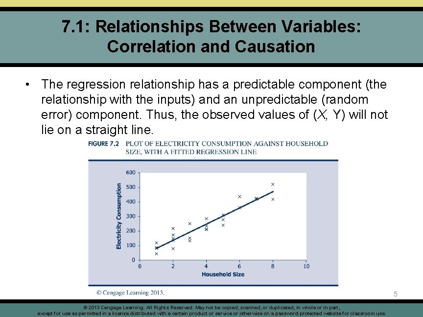
7. 1: Relationships Between Variables: Correlation and Causation • The regression relationship has a predictable component (the relationship with the inputs) and an unpredictable (random error) component. Thus, the observed values of (X, Y) will not lie on a straight line. 5 © 2013 Cengage Learning. All Rights Reserved. May not be copied, scanned, or duplicated, in whole or in part, except for use as permitted in a license distributed with a certain product or service or otherwise on a password-protected website for classroom use.

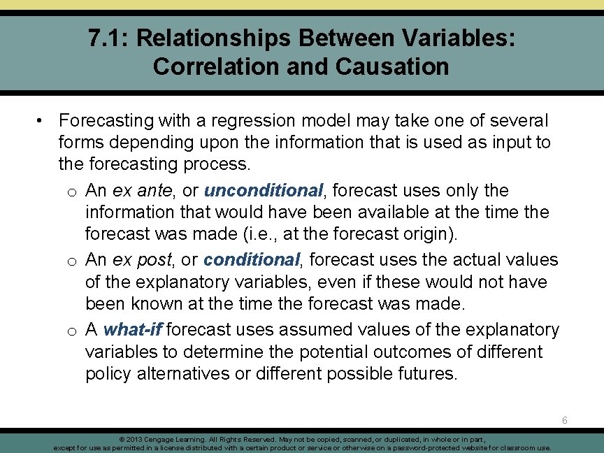
7. 1: Relationships Between Variables: Correlation and Causation • Forecasting with a regression model may take one of several forms depending upon the information that is used as input to the forecasting process. o An ex ante, or unconditional, forecast uses only the information that would have been available at the time the forecast was made (i. e. , at the forecast origin). o An ex post, or conditional, forecast uses the actual values of the explanatory variables, even if these would not have been known at the time the forecast was made. o A what-if forecast uses assumed values of the explanatory variables to determine the potential outcomes of different policy alternatives or different possible futures. 6 © 2013 Cengage Learning. All Rights Reserved. May not be copied, scanned, or duplicated, in whole or in part, except for use as permitted in a license distributed with a certain product or service or otherwise on a password-protected website for classroom use.

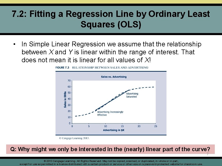
7. 2: Fitting a Regression Line by Ordinary Least Squares (OLS) • In Simple Linear Regression we assume that the relationship between X and Y is linear within the range of interest. That does not mean it is linear for all values of X! Q: Why might we only be interested in the (nearly) linear part of the curve? 7 © 2013 Cengage Learning. All Rights Reserved. May not be copied, scanned, or duplicated, in whole or in part, except for use as permitted in a license distributed with a certain product or service or otherwise on a password-protected website for classroom use.

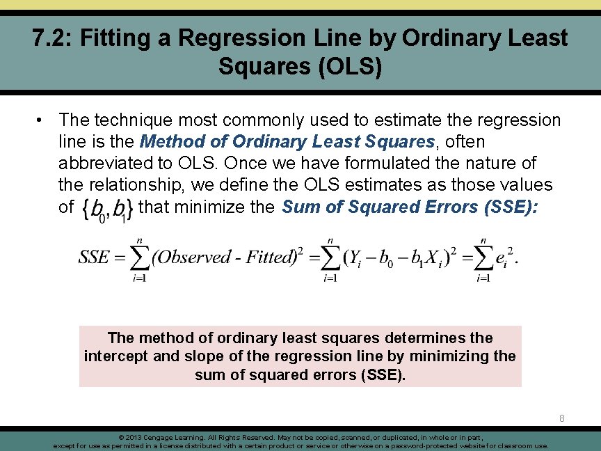
7. 2: Fitting a Regression Line by Ordinary Least Squares (OLS) • The technique most commonly used to estimate the regression line is the Method of Ordinary Least Squares, often abbreviated to OLS. Once we have formulated the nature of the relationship, we define the OLS estimates as those values of that minimize the Sum of Squared Errors (SSE): The method of ordinary least squares determines the intercept and slope of the regression line by minimizing the sum of squared errors (SSE). 8 © 2013 Cengage Learning. All Rights Reserved. May not be copied, scanned, or duplicated, in whole or in part, except for use as permitted in a license distributed with a certain product or service or otherwise on a password-protected website for classroom use.

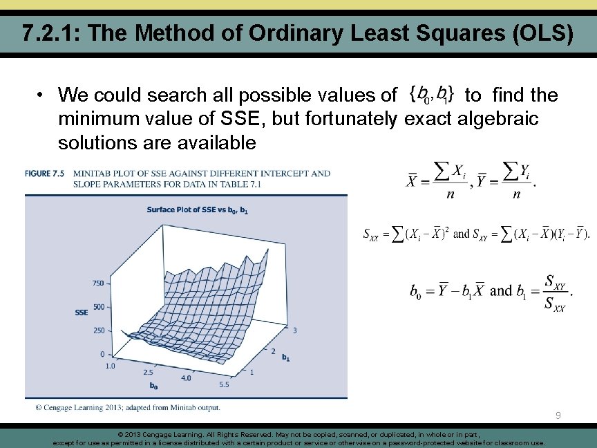
7. 2. 1: The Method of Ordinary Least Squares (OLS) • We could search all possible values of to find the minimum value of SSE, but fortunately exact algebraic solutions are available 9 © 2013 Cengage Learning. All Rights Reserved. May not be copied, scanned, or duplicated, in whole or in part, except for use as permitted in a license distributed with a certain product or service or otherwise on a password-protected website for classroom use.

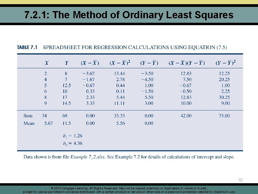
7. 2. 1: The Method of Ordinary Least Squares 10 © 2013 Cengage Learning. All Rights Reserved. May not be copied, scanned, or duplicated, in whole or in part, except for use as permitted in a license distributed with a certain product or service or otherwise on a password-protected website for classroom use.

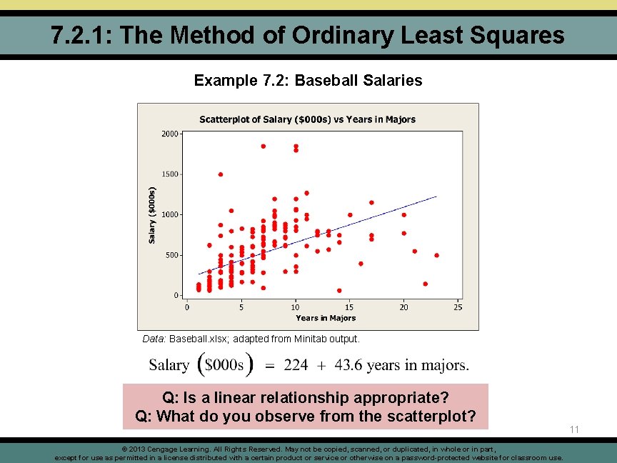
7. 2. 1: The Method of Ordinary Least Squares Example 7. 2: Baseball Salaries Data: Baseball. xlsx; adapted from Minitab output. Q: Is a linear relationship appropriate? Q: What do you observe from the scatterplot? © 2013 Cengage Learning. All Rights Reserved. May not be copied, scanned, or duplicated, in whole or in part, except for use as permitted in a license distributed with a certain product or service or otherwise on a password-protected website for classroom use. 11

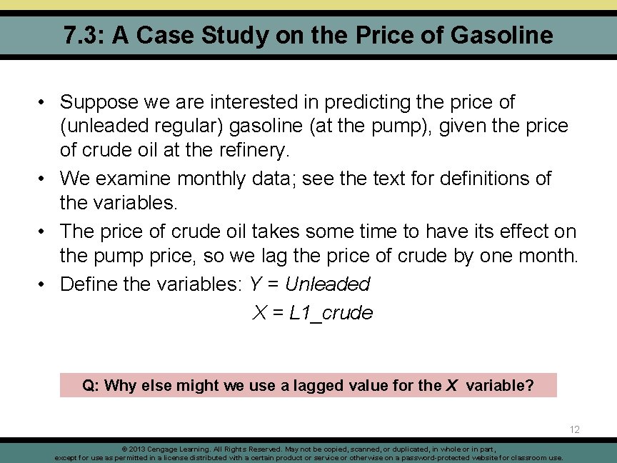
7. 3: A Case Study on the Price of Gasoline • Suppose we are interested in predicting the price of (unleaded regular) gasoline (at the pump), given the price of crude oil at the refinery. • We examine monthly data; see the text for definitions of the variables. • The price of crude oil takes some time to have its effect on the pump price, so we lag the price of crude by one month. • Define the variables: Y = Unleaded X = L 1_crude Q: Why else might we use a lagged value for the X variable? 12 © 2013 Cengage Learning. All Rights Reserved. May not be copied, scanned, or duplicated, in whole or in part, except for use as permitted in a license distributed with a certain product or service or otherwise on a password-protected website for classroom use.

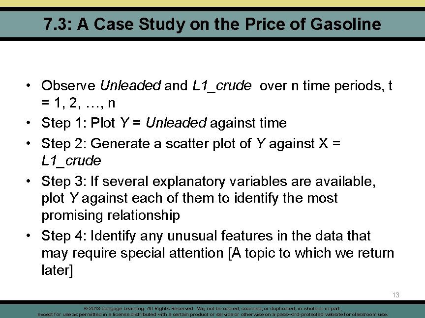
7. 3: A Case Study on the Price of Gasoline • Observe Unleaded and L 1_crude over n time periods, t = 1, 2, …, n • Step 1: Plot Y = Unleaded against time • Step 2: Generate a scatter plot of Y against X = L 1_crude • Step 3: If several explanatory variables are available, plot Y against each of them to identify the most promising relationship • Step 4: Identify any unusual features in the data that may require special attention [A topic to which we return later] 13 © 2013 Cengage Learning. All Rights Reserved. May not be copied, scanned, or duplicated, in whole or in part, except for use as permitted in a license distributed with a certain product or service or otherwise on a password-protected website for classroom use.

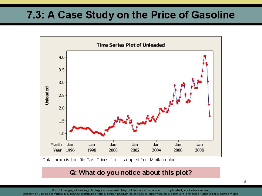
7. 3: A Case Study on the Price of Gasoline Data shown is from file Gas_Prices_1. xlsx; adapted from Minitab output. Q: What do you notice about this plot? 14 © 2013 Cengage Learning. All Rights Reserved. May not be copied, scanned, or duplicated, in whole or in part, except for use as permitted in a license distributed with a certain product or service or otherwise on a password-protected website for classroom use.

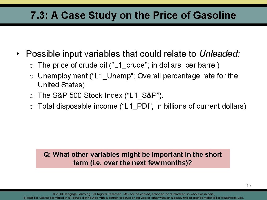
7. 3: A Case Study on the Price of Gasoline • Possible input variables that could relate to Unleaded: o The price of crude oil (“L 1_crude”; in dollars per barrel) o Unemployment (“L 1_Unemp”; Overall percentage rate for the United States) o The S&P 500 Stock Index (“L 1_S&P”). o Total disposable income (“L 1_PDI”; in billions of current dollars) Q: What other variables might be important in the short term (i. e. over the next few months)? 15 © 2013 Cengage Learning. All Rights Reserved. May not be copied, scanned, or duplicated, in whole or in part, except for use as permitted in a license distributed with a certain product or service or otherwise on a password-protected website for classroom use.

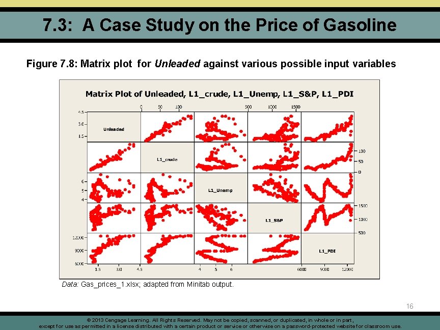
7. 3: A Case Study on the Price of Gasoline Figure 7. 8: Matrix plot for Unleaded against various possible input variables Data: Gas_prices_1. xlsx; adapted from Minitab output. 16 © 2013 Cengage Learning. All Rights Reserved. May not be copied, scanned, or duplicated, in whole or in part, except for use as permitted in a license distributed with a certain product or service or otherwise on a password-protected website for classroom use.

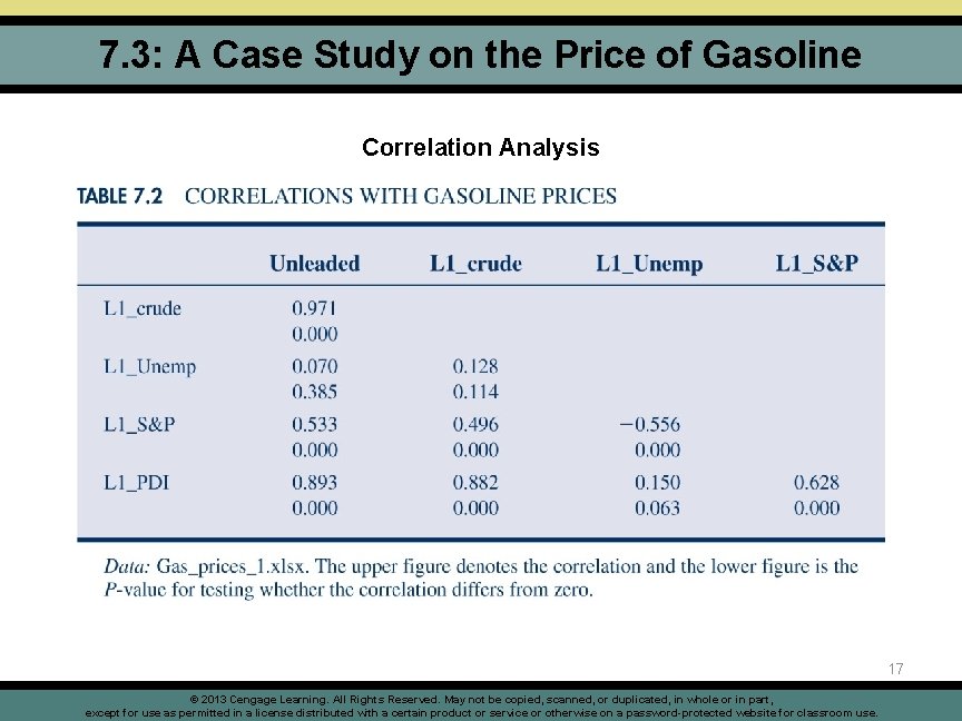
7. 3: A Case Study on the Price of Gasoline Correlation Analysis 17 © 2013 Cengage Learning. All Rights Reserved. May not be copied, scanned, or duplicated, in whole or in part, except for use as permitted in a license distributed with a certain product or service or otherwise on a password-protected website for classroom use.

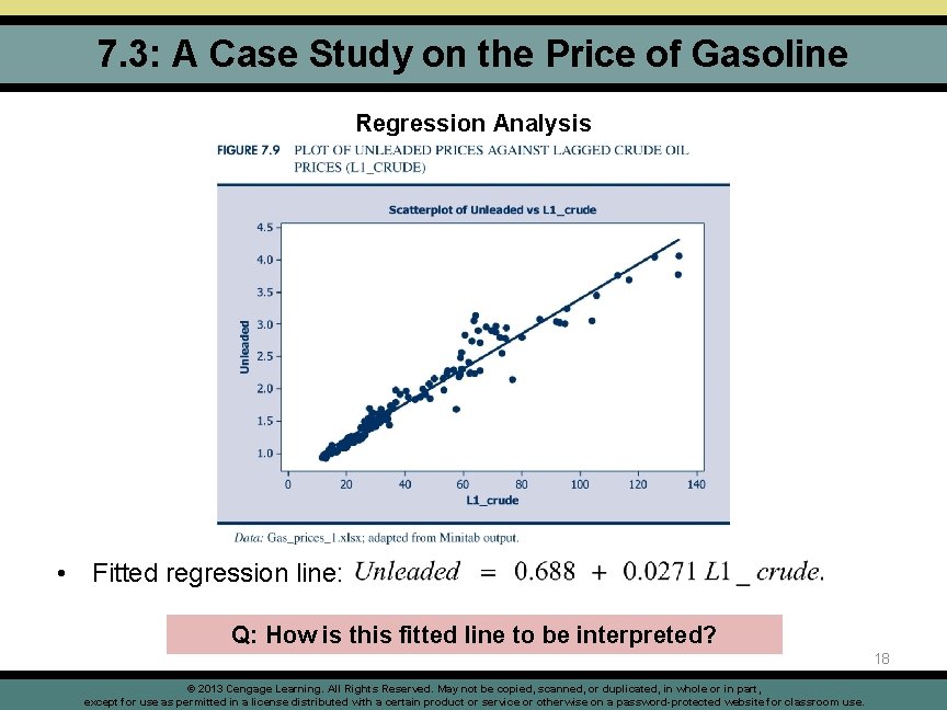
7. 3: A Case Study on the Price of Gasoline Regression Analysis • Fitted regression line: Q: How is this fitted line to be interpreted? 18 © 2013 Cengage Learning. All Rights Reserved. May not be copied, scanned, or duplicated, in whole or in part, except for use as permitted in a license distributed with a certain product or service or otherwise on a password-protected website for classroom use.

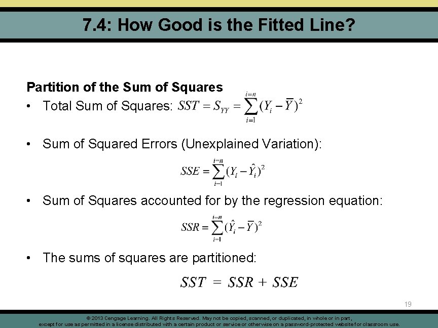
7. 4: How Good is the Fitted Line? Partition of the Sum of Squares • Total Sum of Squares: • Sum of Squared Errors (Unexplained Variation): • Sum of Squares accounted for by the regression equation: • The sums of squares are partitioned: 19 © 2013 Cengage Learning. All Rights Reserved. May not be copied, scanned, or duplicated, in whole or in part, except for use as permitted in a license distributed with a certain product or service or otherwise on a password-protected website for classroom use.

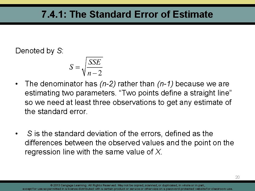
7. 4. 1: The Standard Error of Estimate Denoted by S: • The denominator has (n-2) rather than (n-1) because we are estimating two parameters. “Two points define a straight line” so we need at least three observations to get any estimate of the standard error. • S is the standard deviation of the errors, defined as the differences between the observed values and the point on the regression line with the same value of X. 20 © 2013 Cengage Learning. All Rights Reserved. May not be copied, scanned, or duplicated, in whole or in part, except for use as permitted in a license distributed with a certain product or service or otherwise on a password-protected website for classroom use.

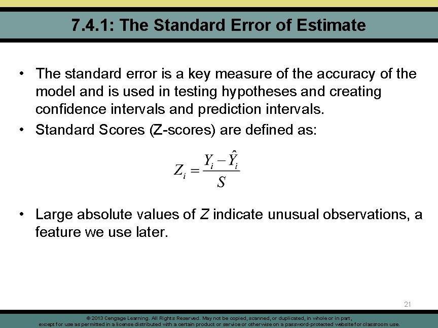
7. 4. 1: The Standard Error of Estimate • The standard error is a key measure of the accuracy of the model and is used in testing hypotheses and creating confidence intervals and prediction intervals. • Standard Scores (Z-scores) are defined as: • Large absolute values of Z indicate unusual observations, a feature we use later. 21 © 2013 Cengage Learning. All Rights Reserved. May not be copied, scanned, or duplicated, in whole or in part, except for use as permitted in a license distributed with a certain product or service or otherwise on a password-protected website for classroom use.

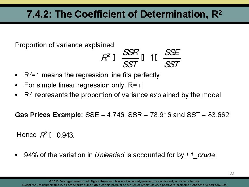
7. 4. 2: The Coefficient of Determination, R 2 Proportion of variance explained: • R 2=1 means the regression line fits perfectly • For simple linear regression only, R=|r| • R 2 represents the proportion of variance explained by the model Gas Prices Example: SSE = 4. 746, SSR = 78. 916 and SST = 83. 662 Hence • 94% of the variation in Unleaded is accounted for by L 1_crude. 22 © 2013 Cengage Learning. All Rights Reserved. May not be copied, scanned, or duplicated, in whole or in part, except for use as permitted in a license distributed with a certain product or service or otherwise on a password-protected website for classroom use.

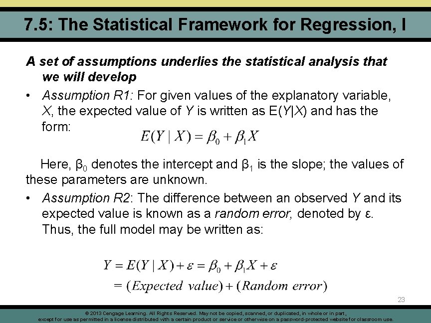
7. 5: The Statistical Framework for Regression, I A set of assumptions underlies the statistical analysis that we will develop • Assumption R 1: For given values of the explanatory variable, X, the expected value of Y is written as E(Y|X) and has the form: Here, β 0 denotes the intercept and β 1 is the slope; the values of these parameters are unknown. • Assumption R 2: The difference between an observed Y and its expected value is known as a random error, denoted by ε. Thus, the full model may be written as: 23 © 2013 Cengage Learning. All Rights Reserved. May not be copied, scanned, or duplicated, in whole or in part, except for use as permitted in a license distributed with a certain product or service or otherwise on a password-protected website for classroom use.

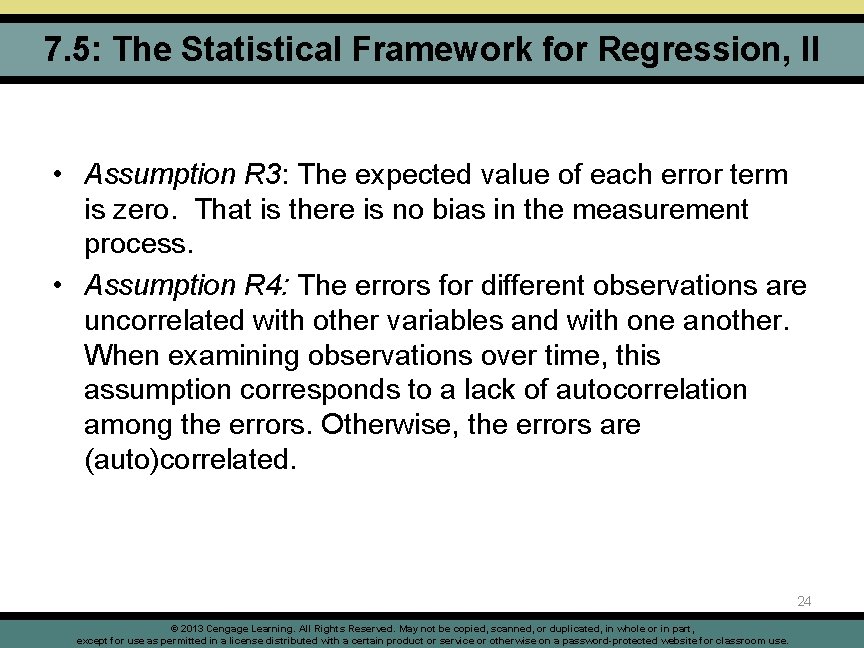
7. 5: The Statistical Framework for Regression, II • Assumption R 3: The expected value of each error term is zero. That is there is no bias in the measurement process. • Assumption R 4: The errors for different observations are uncorrelated with other variables and with one another. When examining observations over time, this assumption corresponds to a lack of autocorrelation among the errors. Otherwise, the errors are (auto)correlated. 24 © 2013 Cengage Learning. All Rights Reserved. May not be copied, scanned, or duplicated, in whole or in part, except for use as permitted in a license distributed with a certain product or service or otherwise on a password-protected website for classroom use.

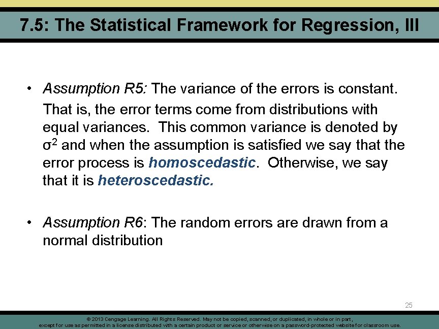
7. 5: The Statistical Framework for Regression, III • Assumption R 5: The variance of the errors is constant. That is, the error terms come from distributions with equal variances. This common variance is denoted by σ2 and when the assumption is satisfied we say that the error process is homoscedastic. Otherwise, we say that it is heteroscedastic. • Assumption R 6: The random errors are drawn from a normal distribution 25 © 2013 Cengage Learning. All Rights Reserved. May not be copied, scanned, or duplicated, in whole or in part, except for use as permitted in a license distributed with a certain product or service or otherwise on a password-protected website for classroom use.

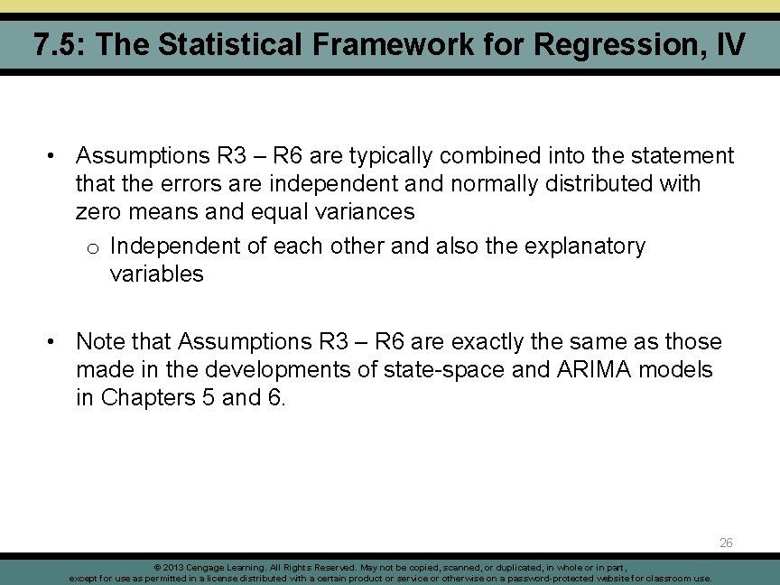
7. 5: The Statistical Framework for Regression, IV • Assumptions R 3 – R 6 are typically combined into the statement that the errors are independent and normally distributed with zero means and equal variances o Independent of each other and also the explanatory variables • Note that Assumptions R 3 – R 6 are exactly the same as those made in the developments of state-space and ARIMA models in Chapters 5 and 6. 26 © 2013 Cengage Learning. All Rights Reserved. May not be copied, scanned, or duplicated, in whole or in part, except for use as permitted in a license distributed with a certain product or service or otherwise on a password-protected website for classroom use.

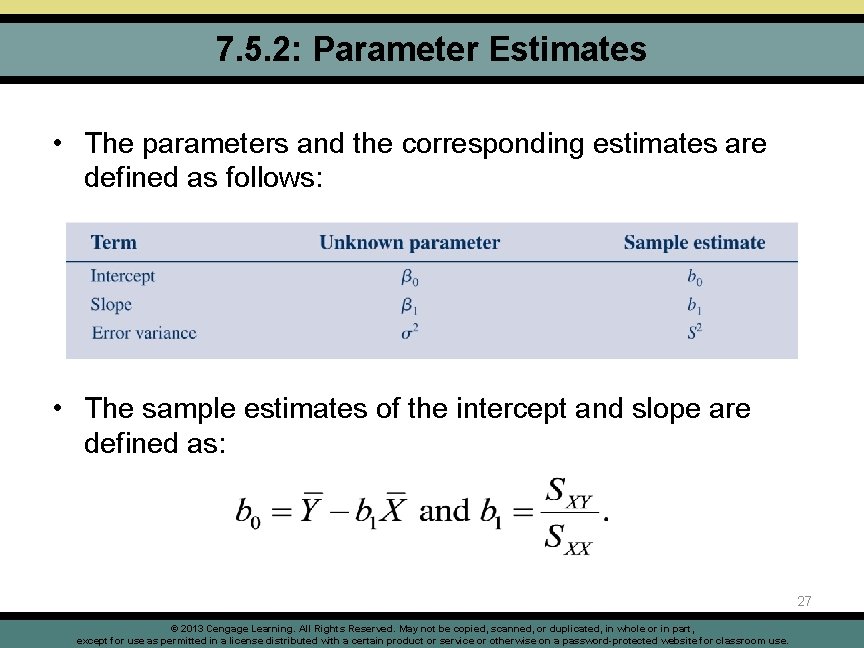
7. 5. 2: Parameter Estimates • The parameters and the corresponding estimates are defined as follows: • The sample estimates of the intercept and slope are defined as: 27 © 2013 Cengage Learning. All Rights Reserved. May not be copied, scanned, or duplicated, in whole or in part, except for use as permitted in a license distributed with a certain product or service or otherwise on a password-protected website for classroom use.

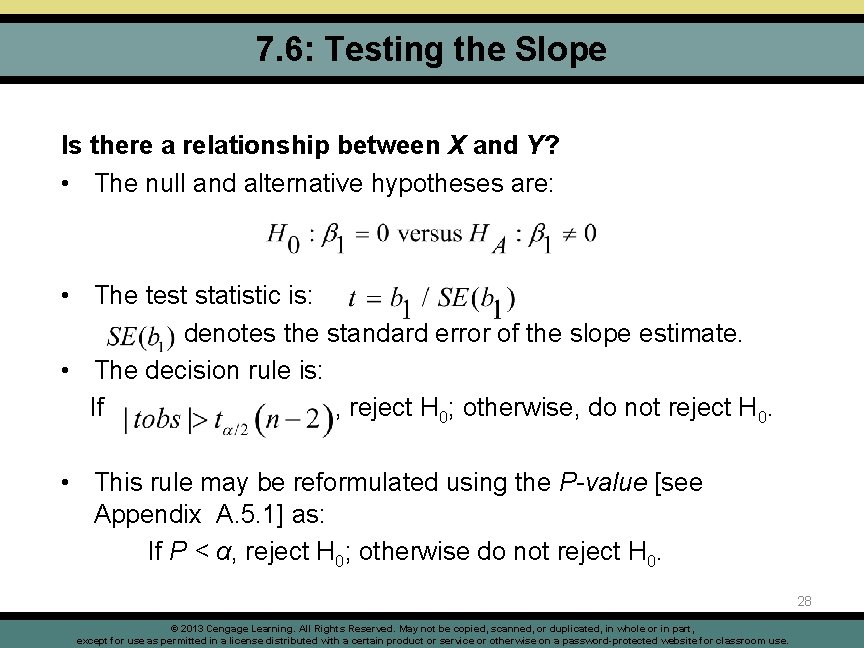
7. 6: Testing the Slope Is there a relationship between X and Y? • The null and alternative hypotheses are: • The test statistic is: denotes the standard error of the slope estimate. • The decision rule is: If , reject H 0; otherwise, do not reject H 0. • This rule may be reformulated using the P-value [see Appendix A. 5. 1] as: If P < α, reject H 0; otherwise do not reject H 0. 28 © 2013 Cengage Learning. All Rights Reserved. May not be copied, scanned, or duplicated, in whole or in part, except for use as permitted in a license distributed with a certain product or service or otherwise on a password-protected website for classroom use.

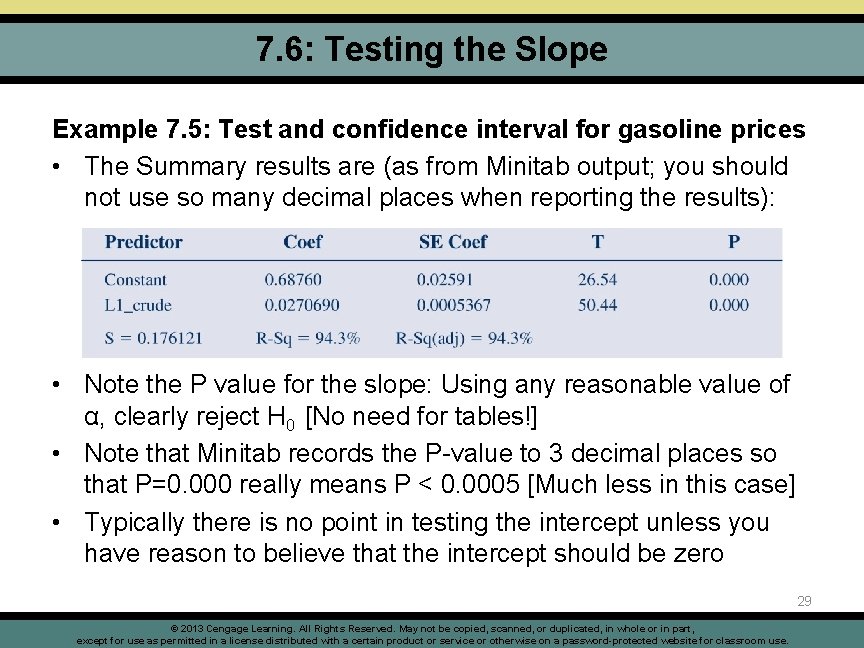
7. 6: Testing the Slope Example 7. 5: Test and confidence interval for gasoline prices • The Summary results are (as from Minitab output; you should not use so many decimal places when reporting the results): • Note the P value for the slope: Using any reasonable value of α, clearly reject H 0 [No need for tables!] • Note that Minitab records the P-value to 3 decimal places so that P=0. 000 really means P < 0. 0005 [Much less in this case] • Typically there is no point in testing the intercept unless you have reason to believe that the intercept should be zero 29 © 2013 Cengage Learning. All Rights Reserved. May not be copied, scanned, or duplicated, in whole or in part, except for use as permitted in a license distributed with a certain product or service or otherwise on a password-protected website for classroom use.

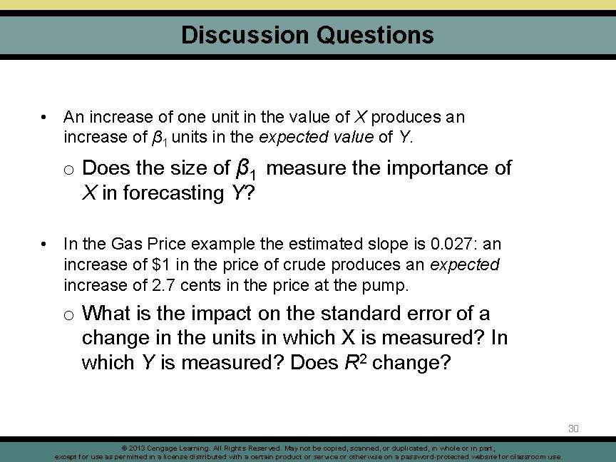
Discussion Questions • An increase of one unit in the value of X produces an increase of β 1 units in the expected value of Y. o Does the size of β 1 measure the importance of X in forecasting Y? • In the Gas Price example the estimated slope is 0. 027: an increase of $1 in the price of crude produces an expected increase of 2. 7 cents in the price at the pump. o What is the impact on the standard error of a change in the units in which X is measured? In which Y is measured? Does R 2 change? 30 © 2013 Cengage Learning. All Rights Reserved. May not be copied, scanned, or duplicated, in whole or in part, except for use as permitted in a license distributed with a certain product or service or otherwise on a password-protected website for classroom use.

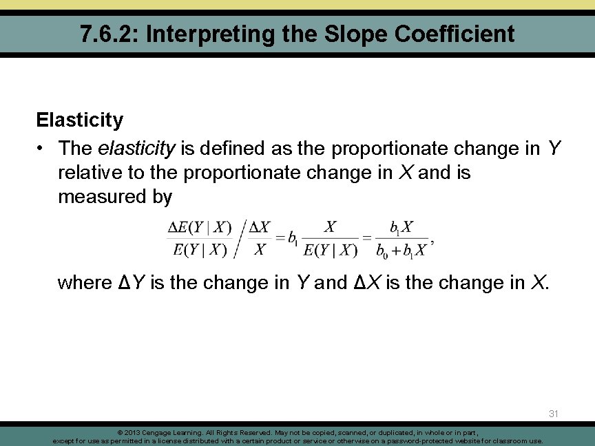
7. 6. 2: Interpreting the Slope Coefficient Elasticity • The elasticity is defined as the proportionate change in Y relative to the proportionate change in X and is measured by where ΔY is the change in Y and ΔX is the change in X. 31 © 2013 Cengage Learning. All Rights Reserved. May not be copied, scanned, or duplicated, in whole or in part, except for use as permitted in a license distributed with a certain product or service or otherwise on a password-protected website for classroom use.

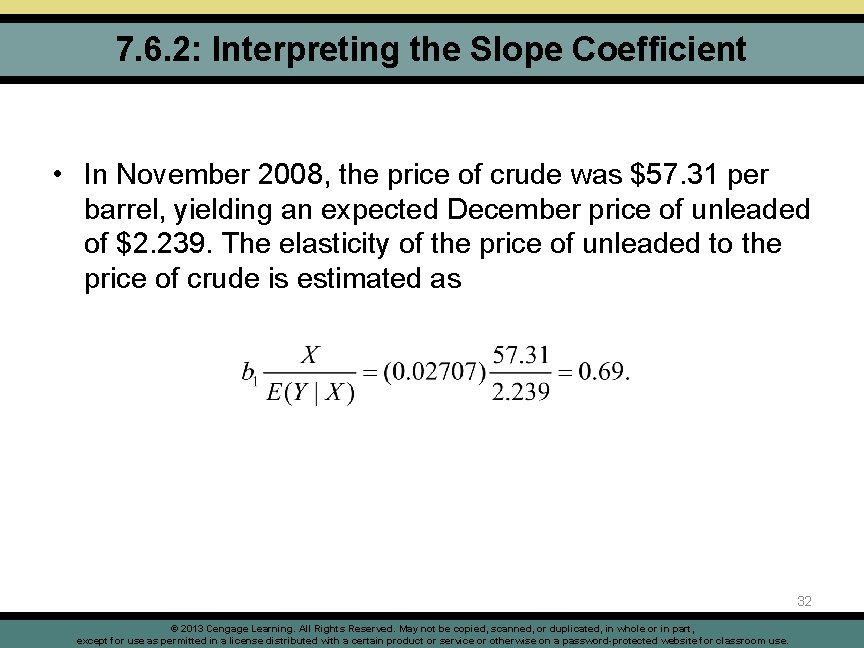
7. 6. 2: Interpreting the Slope Coefficient • In November 2008, the price of crude was $57. 31 per barrel, yielding an expected December price of unleaded of $2. 239. The elasticity of the price of unleaded to the price of crude is estimated as 32 © 2013 Cengage Learning. All Rights Reserved. May not be copied, scanned, or duplicated, in whole or in part, except for use as permitted in a license distributed with a certain product or service or otherwise on a password-protected website for classroom use.

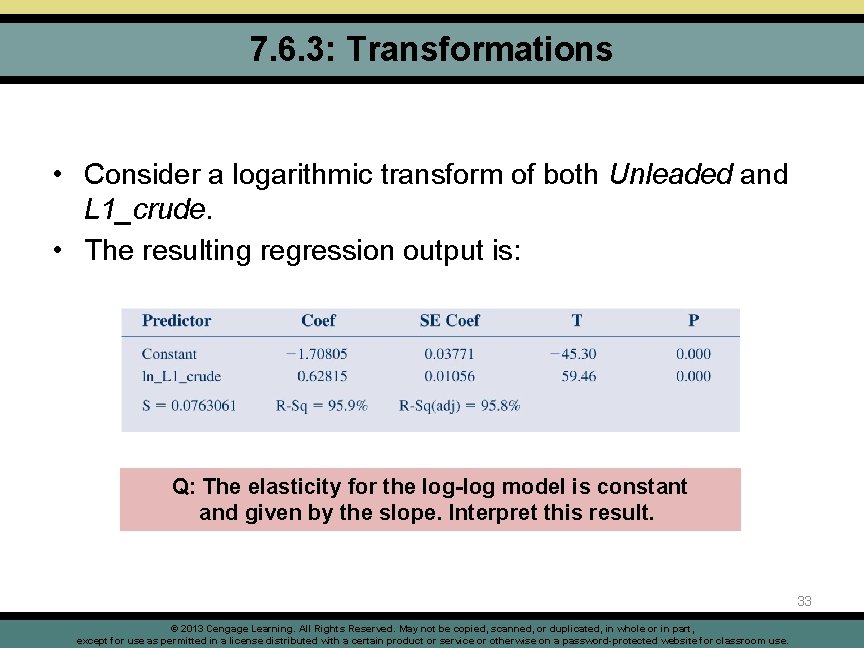
7. 6. 3: Transformations • Consider a logarithmic transform of both Unleaded and L 1_crude. • The resulting regression output is: Q: The elasticity for the log-log model is constant and given by the slope. Interpret this result. 33 © 2013 Cengage Learning. All Rights Reserved. May not be copied, scanned, or duplicated, in whole or in part, except for use as permitted in a license distributed with a certain product or service or otherwise on a password-protected website for classroom use.

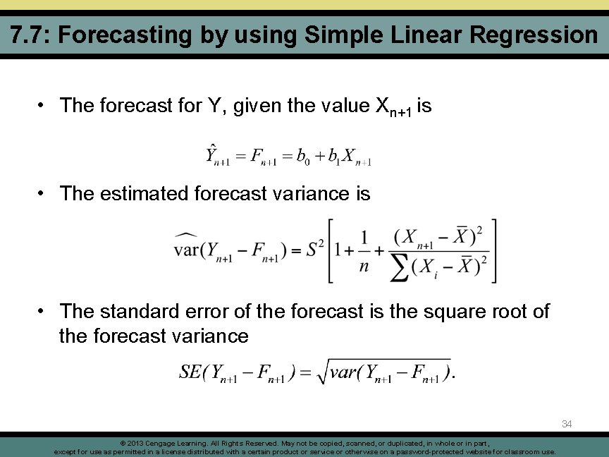
7. 7: Forecasting by using Simple Linear Regression • The forecast for Y, given the value Xn+1 is • The estimated forecast variance is • The standard error of the forecast is the square root of the forecast variance 34 © 2013 Cengage Learning. All Rights Reserved. May not be copied, scanned, or duplicated, in whole or in part, except for use as permitted in a license distributed with a certain product or service or otherwise on a password-protected website for classroom use.

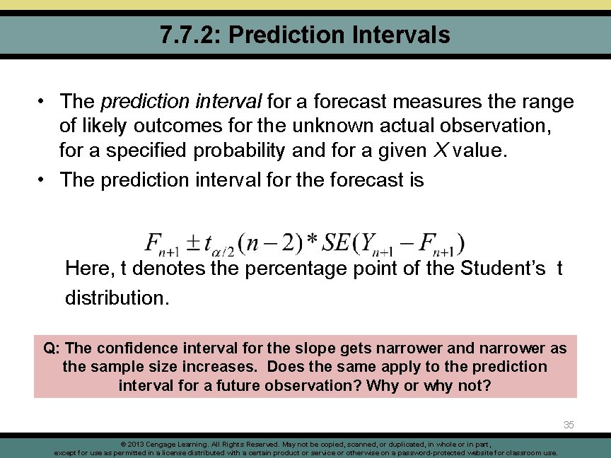
7. 7. 2: Prediction Intervals • The prediction interval for a forecast measures the range of likely outcomes for the unknown actual observation, for a specified probability and for a given X value. • The prediction interval for the forecast is Here, t denotes the percentage point of the Student’s t distribution. Q: The confidence interval for the slope gets narrower and narrower as the sample size increases. Does the same apply to the prediction interval for a future observation? Why or why not? 35 © 2013 Cengage Learning. All Rights Reserved. May not be copied, scanned, or duplicated, in whole or in part, except for use as permitted in a license distributed with a certain product or service or otherwise on a password-protected website for classroom use.

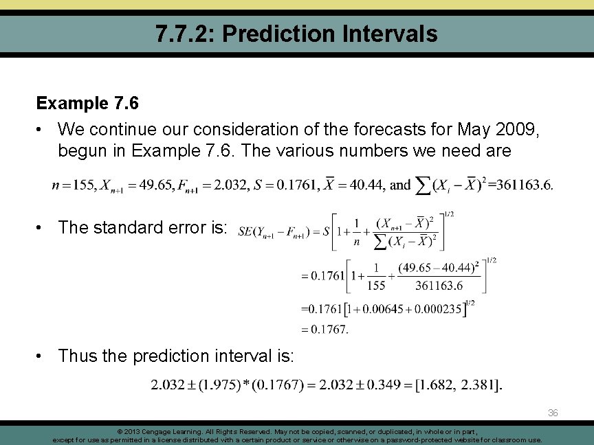
7. 7. 2: Prediction Intervals Example 7. 6 • We continue our consideration of the forecasts for May 2009, begun in Example 7. 6. The various numbers we need are • The standard error is: • Thus the prediction interval is: 36 © 2013 Cengage Learning. All Rights Reserved. May not be copied, scanned, or duplicated, in whole or in part, except for use as permitted in a license distributed with a certain product or service or otherwise on a password-protected website for classroom use.

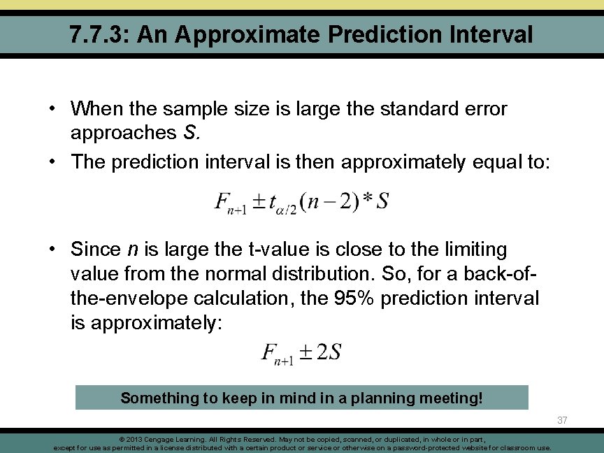
7. 7. 3: An Approximate Prediction Interval • When the sample size is large the standard error approaches S. • The prediction interval is then approximately equal to: • Since n is large the t-value is close to the limiting value from the normal distribution. So, for a back-ofthe-envelope calculation, the 95% prediction interval is approximately: Something to keep in mind in a planning meeting! 37 © 2013 Cengage Learning. All Rights Reserved. May not be copied, scanned, or duplicated, in whole or in part, except for use as permitted in a license distributed with a certain product or service or otherwise on a password-protected website for classroom use.

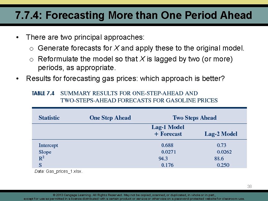
7. 7. 4: Forecasting More than One Period Ahead • There are two principal approaches: o Generate forecasts for X and apply these to the original model. o Reformulate the model so that X is lagged by two (or more) periods, as appropriate. • Results forecasting gas prices: which approach is better? Data: Gas_prices_1. xlsx. 38 © 2013 Cengage Learning. All Rights Reserved. May not be copied, scanned, or duplicated, in whole or in part, except for use as permitted in a license distributed with a certain product or service or otherwise on a password-protected website for classroom use.

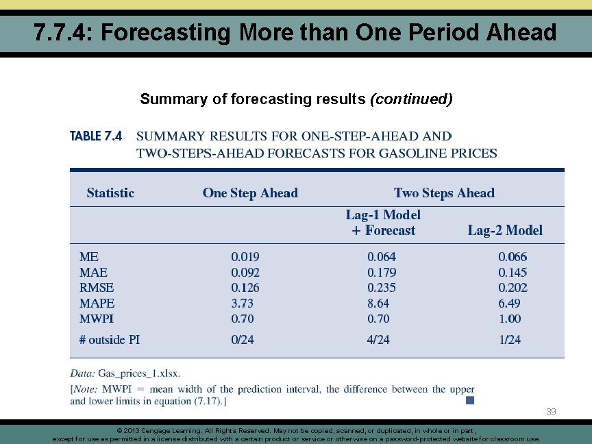
7. 7. 4: Forecasting More than One Period Ahead Summary of forecasting results (continued) 39 © 2013 Cengage Learning. All Rights Reserved. May not be copied, scanned, or duplicated, in whole or in part, except for use as permitted in a license distributed with a certain product or service or otherwise on a password-protected website for classroom use.

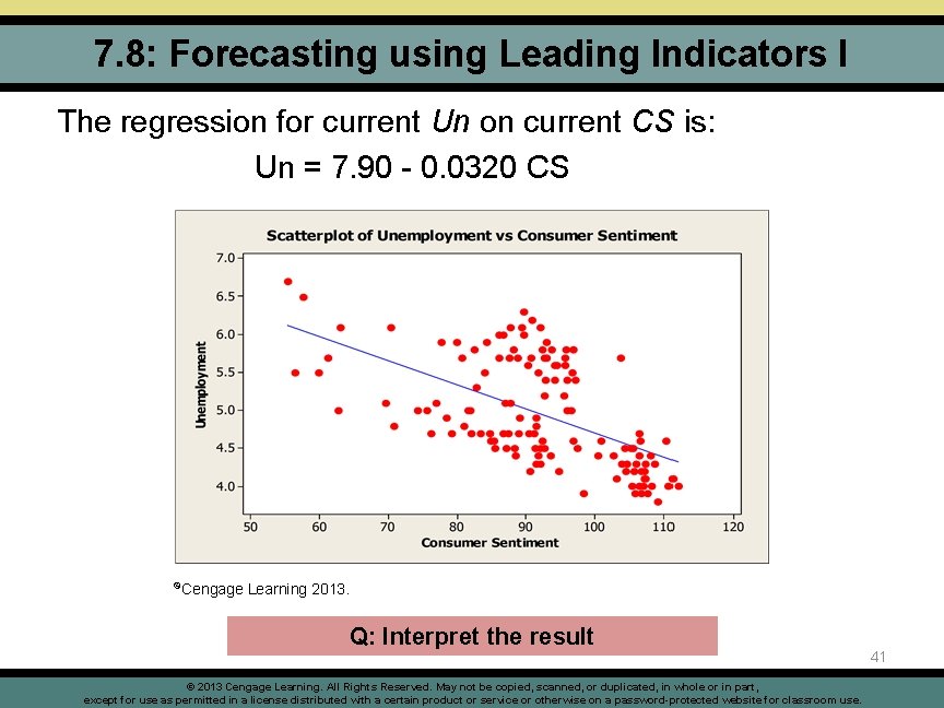
7. 8: Forecasting using Leading Indicators I • Consider the relationship between Unemployment [Un] and Consumer Sentiment [CS] o Monthly data available in Unemp_conconf. xlsx for January 1998 through November 2008; Un is a percentage and CS is measured on the scale (0, 100) ©Cengage Learning 2013. © 2013 Cengage Learning. All Rights Reserved. May not be copied, scanned, or duplicated, in whole or in part, except for use as permitted in a license distributed with a certain product or service or otherwise on a password-protected website for classroom use. 40

7. 8: Forecasting using Leading Indicators I The regression for current Un on current CS is: Un = 7. 90 - 0. 0320 CS ©Cengage Learning 2013. Q: Interpret the result © 2013 Cengage Learning. All Rights Reserved. May not be copied, scanned, or duplicated, in whole or in part, except for use as permitted in a license distributed with a certain product or service or otherwise on a password-protected website for classroom use. 41

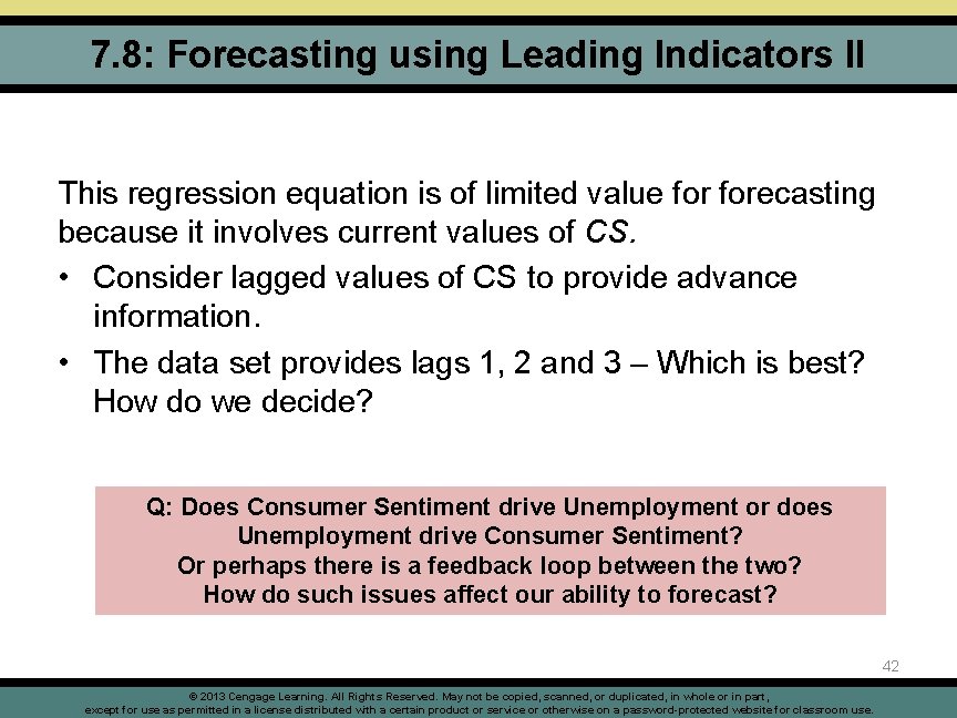
7. 8: Forecasting using Leading Indicators II This regression equation is of limited value forecasting because it involves current values of CS. • Consider lagged values of CS to provide advance information. • The data set provides lags 1, 2 and 3 – Which is best? How do we decide? Q: Does Consumer Sentiment drive Unemployment or does Unemployment drive Consumer Sentiment? Or perhaps there is a feedback loop between the two? How do such issues affect our ability to forecast? 42 © 2013 Cengage Learning. All Rights Reserved. May not be copied, scanned, or duplicated, in whole or in part, except for use as permitted in a license distributed with a certain product or service or otherwise on a password-protected website for classroom use.

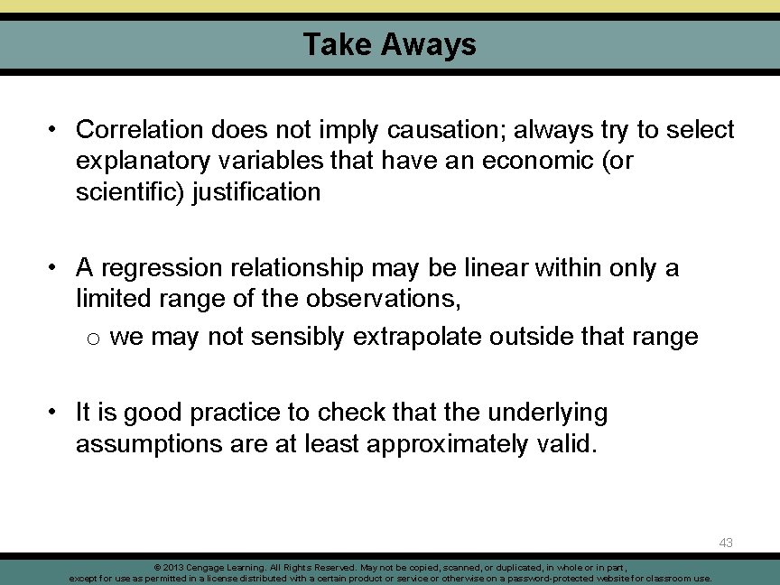
Take Aways • Correlation does not imply causation; always try to select explanatory variables that have an economic (or scientific) justification • A regression relationship may be linear within only a limited range of the observations, o we may not sensibly extrapolate outside that range • It is good practice to check that the underlying assumptions are at least approximately valid. 43 © 2013 Cengage Learning. All Rights Reserved. May not be copied, scanned, or duplicated, in whole or in part, except for use as permitted in a license distributed with a certain product or service or otherwise on a password-protected website for classroom use.

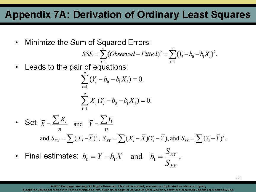
Appendix 7 A: Derivation of Ordinary Least Squares • Minimize the Sum of Squared Errors: • Leads to the pair of equations: • Set • Final estimates: 44 © 2013 Cengage Learning. All Rights Reserved. May not be copied, scanned, or duplicated, in whole or in part, except for use as permitted in a license distributed with a certain product or service or otherwise on a password-protected website for classroom use.