2013 Cengage Learning All Rights Reserved May not

© 2013 Cengage Learning. All Rights Reserved. May not be copied, scanned, or duplicated, in whole or in part, except for use as permitted in a license distributed with a certain product or service or otherwise on a password-protected website for classroom use.

Chapter 6: Autoregressive Integrated Moving Average (ARIMA) Models 6. 1 The Sample Autocorrelation Function 6. 2 Autoregressive Moving Average (ARMA) Models 6. 3 Partial Autocorrelations and Model Selection 6. 4 Model Estimation and Selection 6. 5 Model Diagnostics 6. 6 Outliers 6. 7 Forecasting with ARIMA Models 6. 8 Seasonal ARIMA Models 6. 9 State-Space and ARIMA Models 6. 10 GARCH Models 6. 11 Principles of ARIMA Modeling © 2013 Cengage Learning. All Rights Reserved. May not be copied, scanned, or duplicated, in whole or in part, except for use as permitted in a license distributed with a certain product or service or otherwise on a password-protected website for classroom use. 2

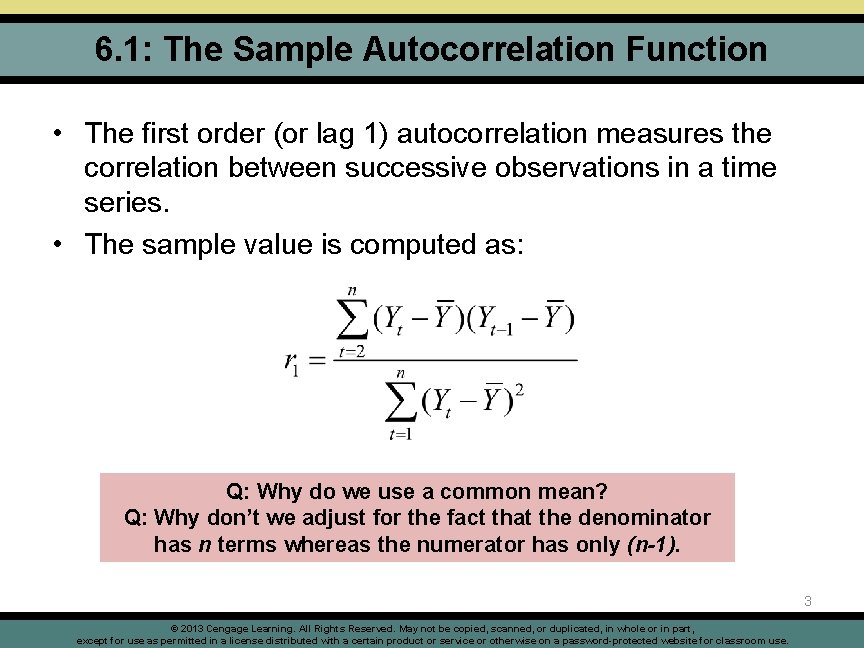
6. 1: The Sample Autocorrelation Function • The first order (or lag 1) autocorrelation measures the correlation between successive observations in a time series. • The sample value is computed as: Q: Why do we use a common mean? Q: Why don’t we adjust for the fact that the denominator has n terms whereas the numerator has only (n-1). 3 © 2013 Cengage Learning. All Rights Reserved. May not be copied, scanned, or duplicated, in whole or in part, except for use as permitted in a license distributed with a certain product or service or otherwise on a password-protected website for classroom use.

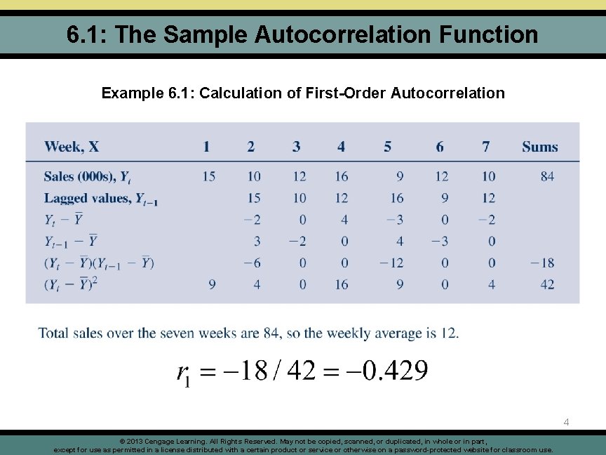
6. 1: The Sample Autocorrelation Function Example 6. 1: Calculation of First-Order Autocorrelation 4 © 2013 Cengage Learning. All Rights Reserved. May not be copied, scanned, or duplicated, in whole or in part, except for use as permitted in a license distributed with a certain product or service or otherwise on a password-protected website for classroom use.

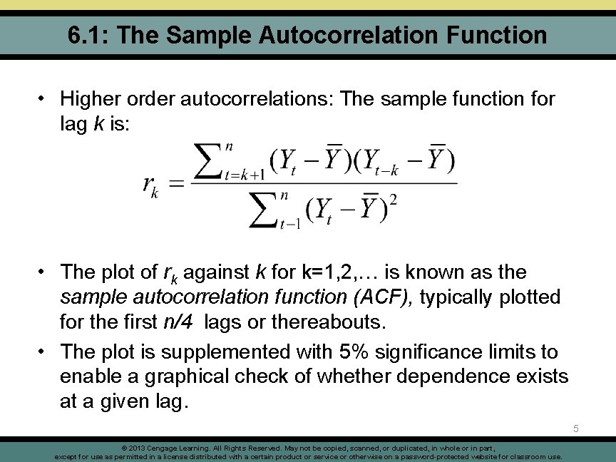
6. 1: The Sample Autocorrelation Function • Higher order autocorrelations: The sample function for lag k is: • The plot of rk against k for k=1, 2, … is known as the sample autocorrelation function (ACF), typically plotted for the first n/4 lags or thereabouts. • The plot is supplemented with 5% significance limits to enable a graphical check of whether dependence exists at a given lag. 5 © 2013 Cengage Learning. All Rights Reserved. May not be copied, scanned, or duplicated, in whole or in part, except for use as permitted in a license distributed with a certain product or service or otherwise on a password-protected website for classroom use.

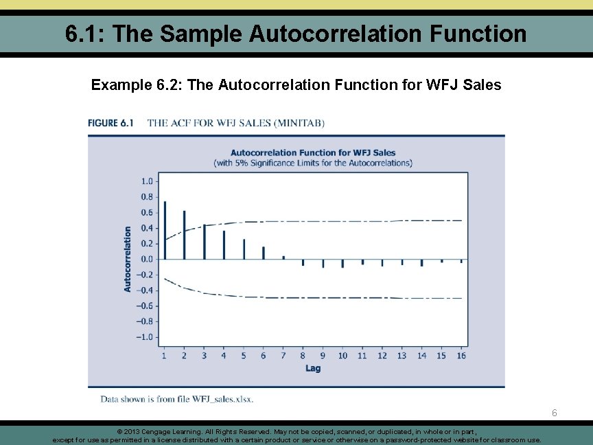
6. 1: The Sample Autocorrelation Function Example 6. 2: The Autocorrelation Function for WFJ Sales 6 © 2013 Cengage Learning. All Rights Reserved. May not be copied, scanned, or duplicated, in whole or in part, except for use as permitted in a license distributed with a certain product or service or otherwise on a password-protected website for classroom use.

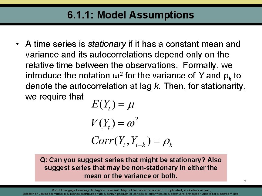
6. 1. 1: Model Assumptions • A time series is stationary if it has a constant mean and variance and its autocorrelations depend only on the relative time between the observations. Formally, we introduce the notation ω2 for the variance of Y and ρk to denote the autocorrelation at lag k. Then, for stationarity, we require that Q: Can you suggest series that might be stationary? Also suggest series that may be non-stationary in either the mean or the variance or both. © 2013 Cengage Learning. All Rights Reserved. May not be copied, scanned, or duplicated, in whole or in part, except for use as permitted in a license distributed with a certain product or service or otherwise on a password-protected website for classroom use. 7

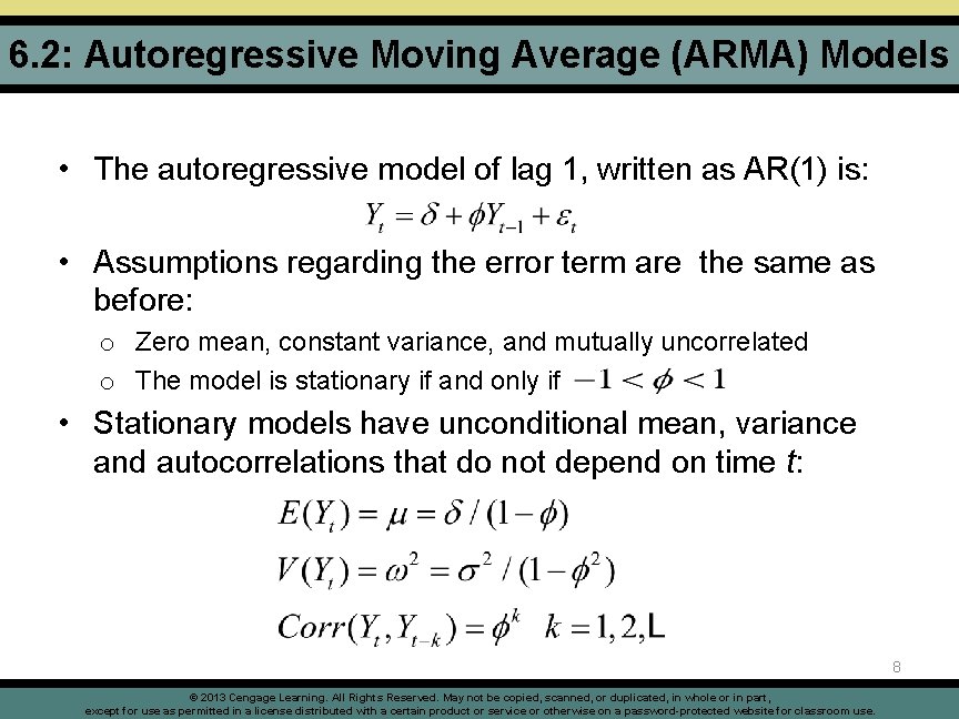
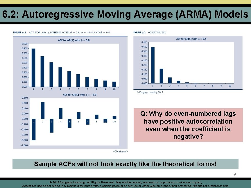
6. 2: Autoregressive Moving Average (ARMA) Models • The autoregressive model of lag 1, written as AR(1) is: • Assumptions regarding the error term are the same as before: o Zero mean, constant variance, and mutually uncorrelated o The model is stationary if and only if • Stationary models have unconditional mean, variance and autocorrelations that do not depend on time t: 8 © 2013 Cengage Learning. All Rights Reserved. May not be copied, scanned, or duplicated, in whole or in part, except for use as permitted in a license distributed with a certain product or service or otherwise on a password-protected website for classroom use.

6. 2: Autoregressive Moving Average (ARMA) Models Q: Why do even-numbered lags have positive autocorrelation even when the coefficient is negative? Sample ACFs will not look exactly like theoretical forms! 9 © 2013 Cengage Learning. All Rights Reserved. May not be copied, scanned, or duplicated, in whole or in part, except for use as permitted in a license distributed with a certain product or service or otherwise on a password-protected website for classroom use.

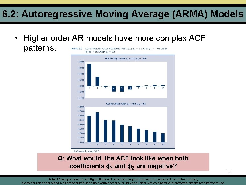
6. 2: Autoregressive Moving Average (ARMA) Models • Higher order AR models have more complex ACF patterns. Q: What would the ACF look like when both coefficients ϕ 1 and ϕ 2 are negative? © 2013 Cengage Learning. All Rights Reserved. May not be copied, scanned, or duplicated, in whole or in part, except for use as permitted in a license distributed with a certain product or service or otherwise on a password-protected website for classroom use. 10

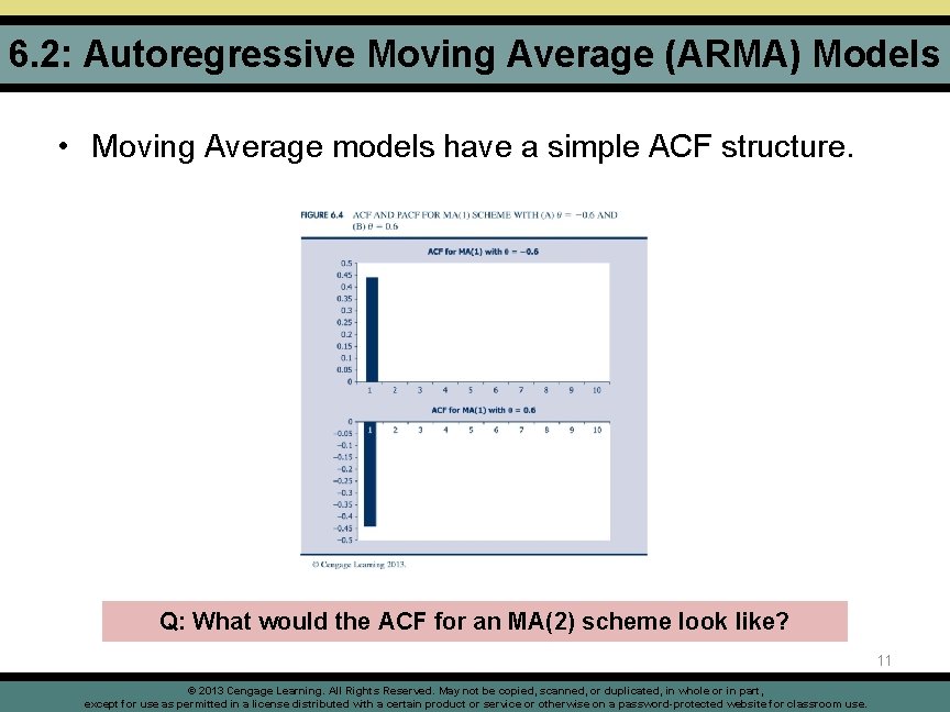
6. 2: Autoregressive Moving Average (ARMA) Models • Moving Average models have a simple ACF structure. Q: What would the ACF for an MA(2) scheme look like? 11 © 2013 Cengage Learning. All Rights Reserved. May not be copied, scanned, or duplicated, in whole or in part, except for use as permitted in a license distributed with a certain product or service or otherwise on a password-protected website for classroom use.

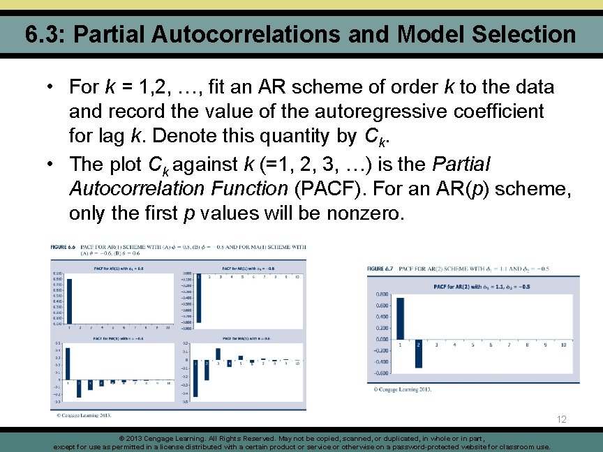
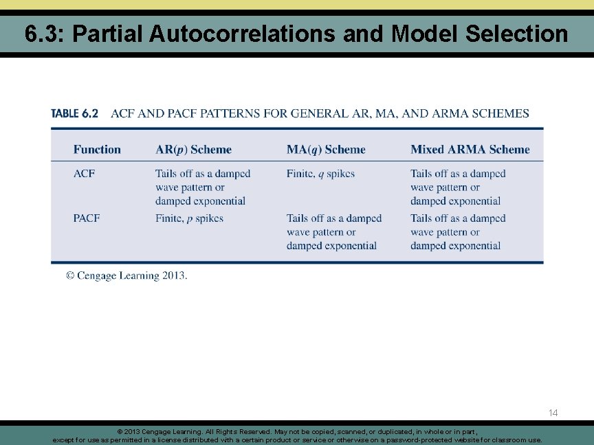
6. 3: Partial Autocorrelations and Model Selection • For k = 1, 2, …, fit an AR scheme of order k to the data and record the value of the autoregressive coefficient for lag k. Denote this quantity by Ck. • The plot Ck against k (=1, 2, 3, …) is the Partial Autocorrelation Function (PACF). For an AR(p) scheme, only the first p values will be nonzero. 12 © 2013 Cengage Learning. All Rights Reserved. May not be copied, scanned, or duplicated, in whole or in part, except for use as permitted in a license distributed with a certain product or service or otherwise on a password-protected website for classroom use.

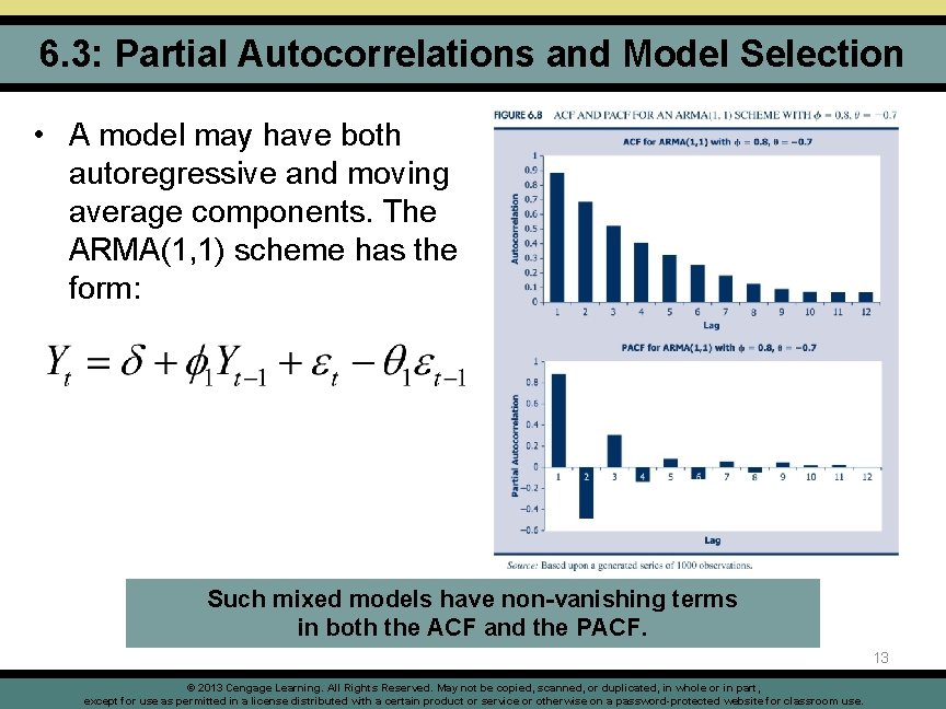
6. 3: Partial Autocorrelations and Model Selection • A model may have both autoregressive and moving average components. The ARMA(1, 1) scheme has the form: . Such mixed models have non-vanishing terms in both the ACF and the PACF. 13 © 2013 Cengage Learning. All Rights Reserved. May not be copied, scanned, or duplicated, in whole or in part, except for use as permitted in a license distributed with a certain product or service or otherwise on a password-protected website for classroom use.

6. 3: Partial Autocorrelations and Model Selection 14 © 2013 Cengage Learning. All Rights Reserved. May not be copied, scanned, or duplicated, in whole or in part, except for use as permitted in a license distributed with a certain product or service or otherwise on a password-protected website for classroom use.

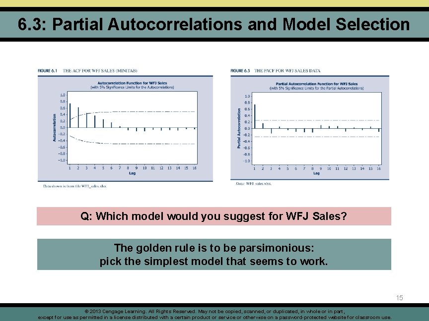
6. 3: Partial Autocorrelations and Model Selection Q: Which model would you suggest for WFJ Sales? The golden rule is to be parsimonious: pick the simplest model that seems to work. 15 © 2013 Cengage Learning. All Rights Reserved. May not be copied, scanned, or duplicated, in whole or in part, except for use as permitted in a license distributed with a certain product or service or otherwise on a password-protected website for classroom use.

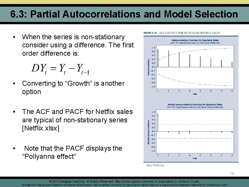
6. 3: Partial Autocorrelations and Model Selection • When the series is non-stationary consider using a difference. The first order difference is: • Converting to “Growth” is another option • The ACF and PACF for Netflix sales are typical of non-stationary series [Netflix. xlsx] • Note that the PACF displays the “Pollyanna effect” 16 © 2013 Cengage Learning. All Rights Reserved. May not be copied, scanned, or duplicated, in whole or in part, except for use as permitted in a license distributed with a certain product or service or otherwise on a password-protected website for classroom use.

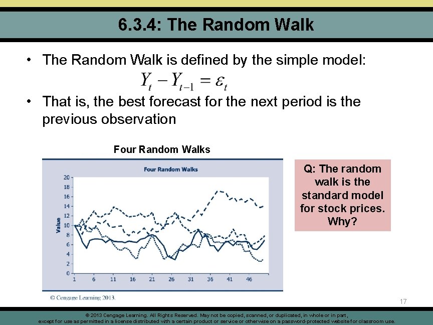
6. 3. 4: The Random Walk • The Random Walk is defined by the simple model: • That is, the best forecast for the next period is the previous observation Four Random Walks Q: The random walk is the standard model for stock prices. Why? 17 © 2013 Cengage Learning. All Rights Reserved. May not be copied, scanned, or duplicated, in whole or in part, except for use as permitted in a license distributed with a certain product or service or otherwise on a password-protected website for classroom use.

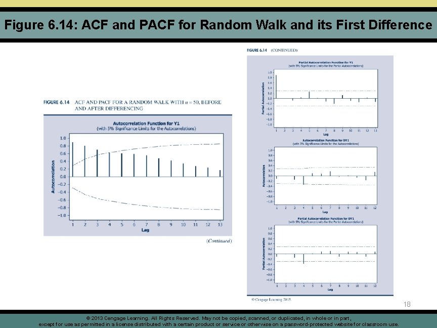
Figure 6. 14: ACF and PACF for Random Walk and its First Difference 18 © 2013 Cengage Learning. All Rights Reserved. May not be copied, scanned, or duplicated, in whole or in part, except for use as permitted in a license distributed with a certain product or service or otherwise on a password-protected website for classroom use.

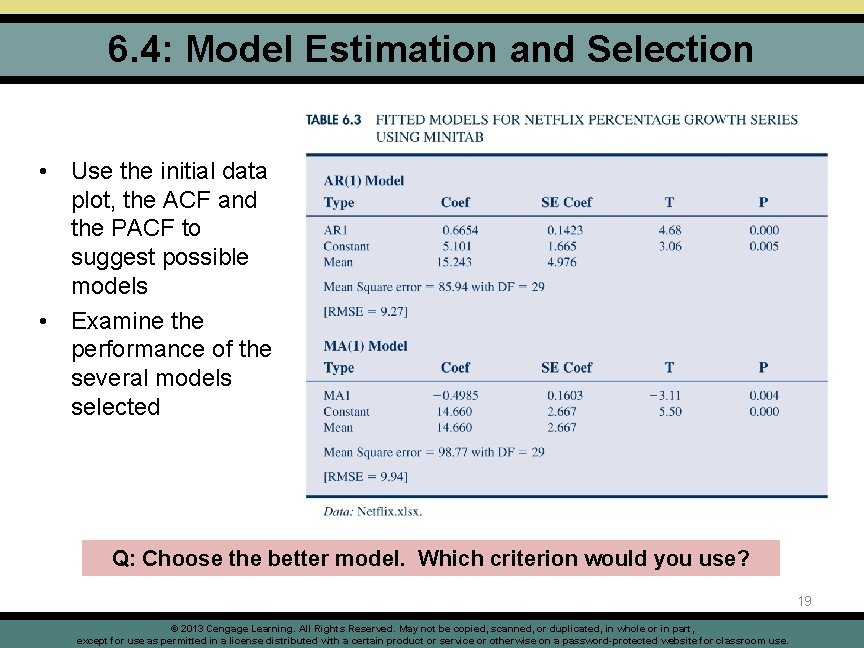
6. 4: Model Estimation and Selection • Use the initial data plot, the ACF and the PACF to suggest possible models • Examine the performance of the several models selected Q: Choose the better model. Which criterion would you use? 19 © 2013 Cengage Learning. All Rights Reserved. May not be copied, scanned, or duplicated, in whole or in part, except for use as permitted in a license distributed with a certain product or service or otherwise on a password-protected website for classroom use.

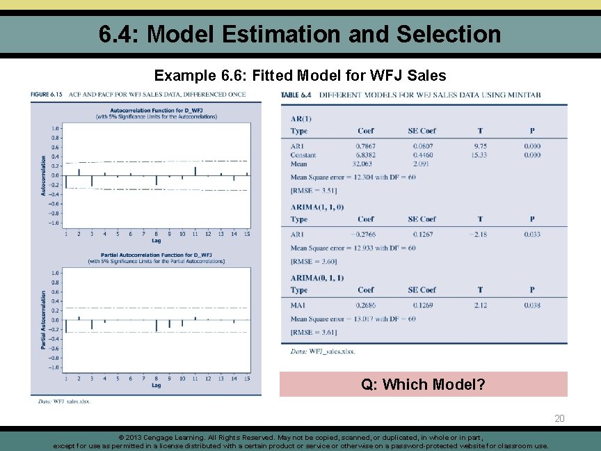
6. 4: Model Estimation and Selection Example 6. 6: Fitted Model for WFJ Sales Q: Which Model? 20 © 2013 Cengage Learning. All Rights Reserved. May not be copied, scanned, or duplicated, in whole or in part, except for use as permitted in a license distributed with a certain product or service or otherwise on a password-protected website for classroom use.

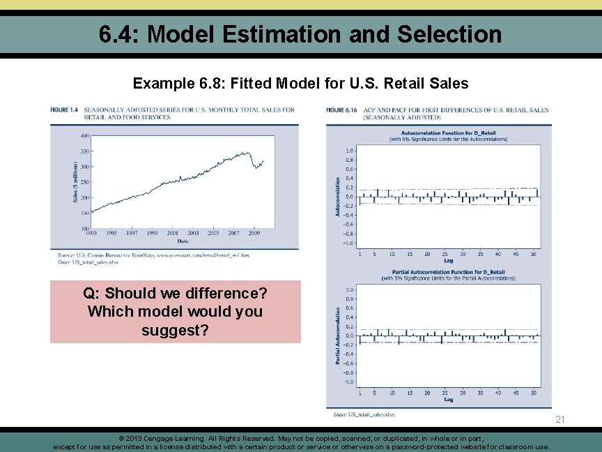
6. 4: Model Estimation and Selection Example 6. 8: Fitted Model for U. S. Retail Sales Q: Should we difference? Which model would you suggest? 21 © 2013 Cengage Learning. All Rights Reserved. May not be copied, scanned, or duplicated, in whole or in part, except for use as permitted in a license distributed with a certain product or service or otherwise on a password-protected website for classroom use.

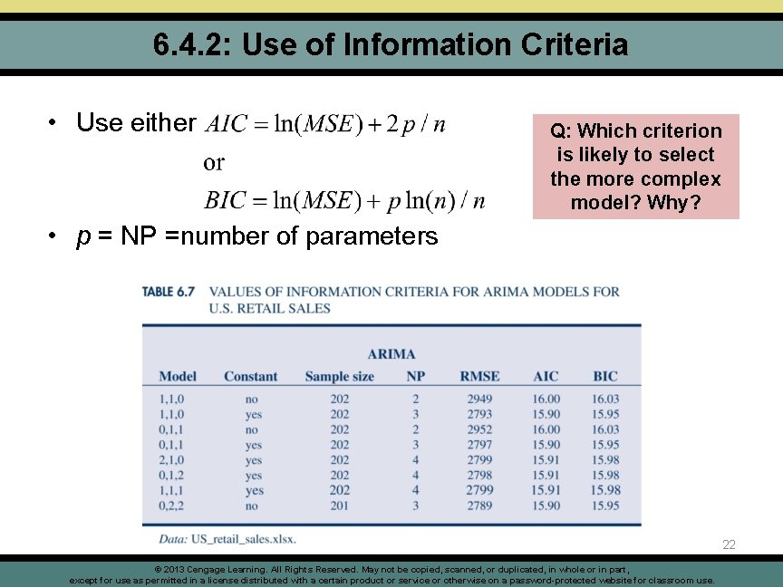
6. 4. 2: Use of Information Criteria • Use either Q: Which criterion is likely to select the more complex model? Why? • p = NP =number of parameters 22 © 2013 Cengage Learning. All Rights Reserved. May not be copied, scanned, or duplicated, in whole or in part, except for use as permitted in a license distributed with a certain product or service or otherwise on a password-protected website for classroom use.

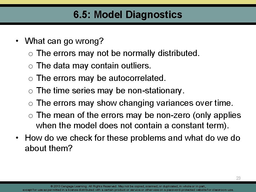
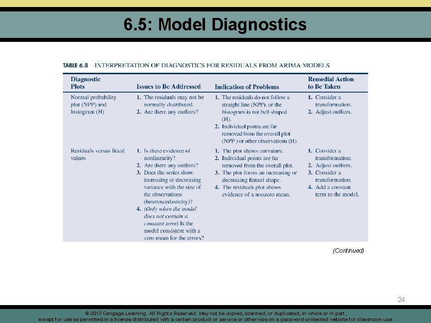
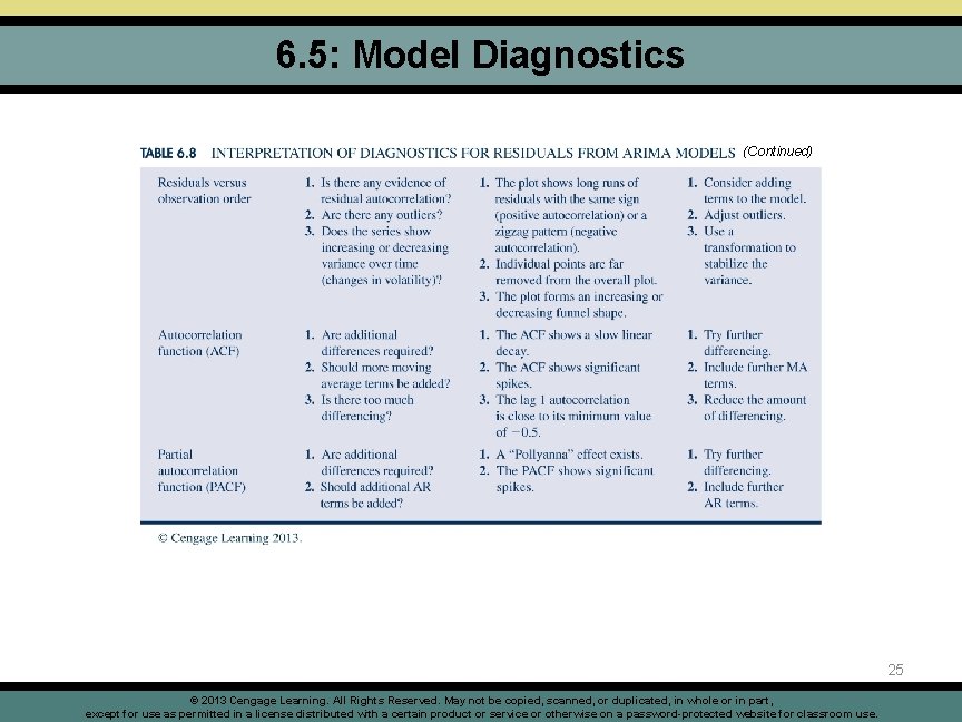
6. 5: Model Diagnostics • What can go wrong? o The errors may not be normally distributed. o The data may contain outliers. o The errors may be autocorrelated. o The time series may be non-stationary. o The errors may show changing variances over time. o The mean of the errors may be non-zero (only applies when the model does not contain a constant term). • How do we check for these problems and what do we do about them? 23 © 2013 Cengage Learning. All Rights Reserved. May not be copied, scanned, or duplicated, in whole or in part, except for use as permitted in a license distributed with a certain product or service or otherwise on a password-protected website for classroom use.

6. 5: Model Diagnostics (Continued) 24 © 2013 Cengage Learning. All Rights Reserved. May not be copied, scanned, or duplicated, in whole or in part, except for use as permitted in a license distributed with a certain product or service or otherwise on a password-protected website for classroom use.

6. 5: Model Diagnostics (Continued) 25 © 2013 Cengage Learning. All Rights Reserved. May not be copied, scanned, or duplicated, in whole or in part, except for use as permitted in a license distributed with a certain product or service or otherwise on a password-protected website for classroom use.

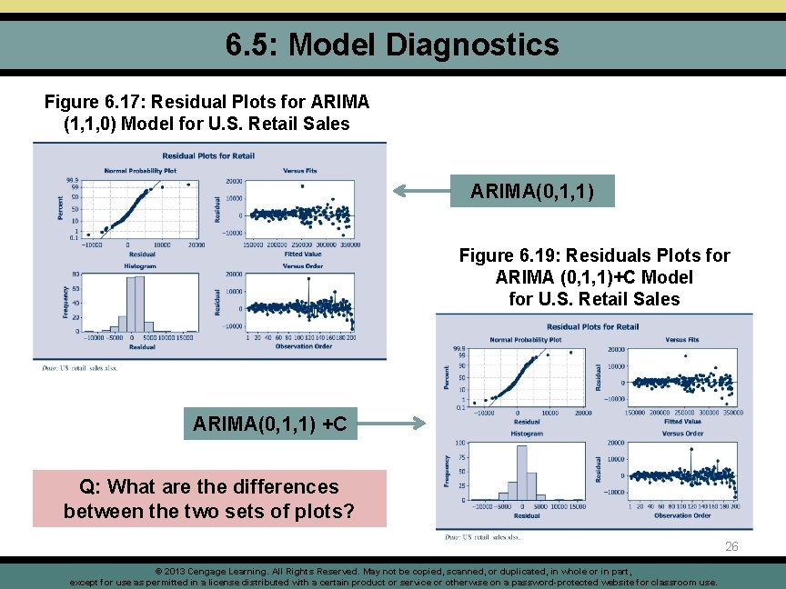
6. 5: Model Diagnostics Figure 6. 17: Residual Plots for ARIMA (1, 1, 0) Model for U. S. Retail Sales ARIMA(0, 1, 1) Figure 6. 19: Residuals Plots for ARIMA (0, 1, 1)+C Model for U. S. Retail Sales ARIMA(0, 1, 1) +C Q: What are the differences between the two sets of plots? 26 © 2013 Cengage Learning. All Rights Reserved. May not be copied, scanned, or duplicated, in whole or in part, except for use as permitted in a license distributed with a certain product or service or otherwise on a password-protected website for classroom use.

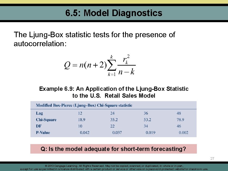
6. 5: Model Diagnostics The Ljung-Box statistic tests for the presence of autocorrelation: Example 6. 9: An Application of the Ljung-Box Statistic to the U. S. Retail Sales Model Q: Is the model adequate for short-term forecasting? 27 © 2013 Cengage Learning. All Rights Reserved. May not be copied, scanned, or duplicated, in whole or in part, except for use as permitted in a license distributed with a certain product or service or otherwise on a password-protected website for classroom use.

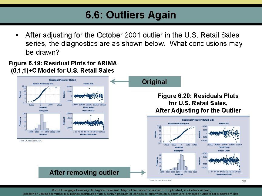
6. 6: Outliers Again • After adjusting for the October 2001 outlier in the U. S. Retail Sales series, the diagnostics are as shown below. What conclusions may be drawn? Figure 6. 19: Residual Plots for ARIMA (0, 1, 1)+C Model for U. S. Retail Sales Original Figure 6. 20: Residuals Plots for U. S. Retail Sales, After Adjusting for the Outlier After removing outlier 28 © 2013 Cengage Learning. All Rights Reserved. May not be copied, scanned, or duplicated, in whole or in part, except for use as permitted in a license distributed with a certain product or service or otherwise on a password-protected website for classroom use.

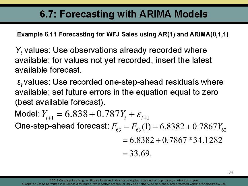
6. 7: Forecasting with ARIMA Models Example 6. 11 Forecasting for WFJ Sales using AR(1) and ARIMA(0, 1, 1) Yt values: Use observations already recorded where available; for values not yet recorded, insert the latest available forecast. εt values: Use recorded one-step-ahead residuals where available; set future errors in the equation equal to zero (best available forecast). Model: One-step-ahead forecast: 29 © 2013 Cengage Learning. All Rights Reserved. May not be copied, scanned, or duplicated, in whole or in part, except for use as permitted in a license distributed with a certain product or service or otherwise on a password-protected website for classroom use.

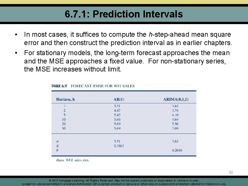
6. 7. 1: Prediction Intervals • In most cases, it suffices to compute the h-step-ahead mean square error and then construct the prediction interval as in earlier chapters. • For stationary models, the long-term forecast approaches the mean and the MSE approaches a fixed value. For non-stationary series, the MSE increases without limit. 30 © 2013 Cengage Learning. All Rights Reserved. May not be copied, scanned, or duplicated, in whole or in part, except for use as permitted in a license distributed with a certain product or service or otherwise on a password-protected website for classroom use.

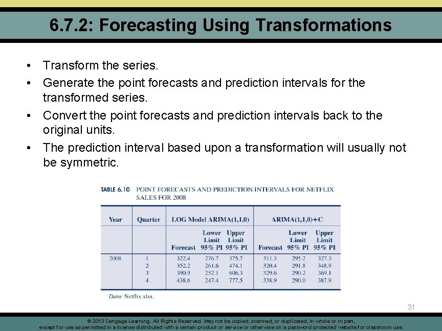
6. 7. 2: Forecasting Using Transformations • Transform the series. • Generate the point forecasts and prediction intervals for the transformed series. • Convert the point forecasts and prediction intervals back to the original units. • The prediction interval based upon a transformation will usually not be symmetric. 31 © 2013 Cengage Learning. All Rights Reserved. May not be copied, scanned, or duplicated, in whole or in part, except for use as permitted in a license distributed with a certain product or service or otherwise on a password-protected website for classroom use.

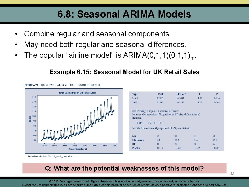
6. 8: Seasonal ARIMA Models • Combine regular and seasonal components. • May need both regular and seasonal differences. • The popular “airline model” is ARIMA(0, 1, 1)m. Example 6. 15: Seasonal Model for UK Retail Sales Q: What are the potential weaknesses of this model? © 2013 Cengage Learning. All Rights Reserved. May not be copied, scanned, or duplicated, in whole or in part, except for use as permitted in a license distributed with a certain product or service or otherwise on a password-protected website for classroom use. 32

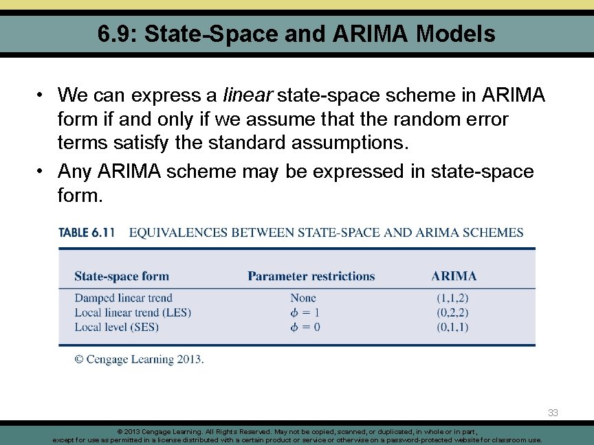
6. 9: State-Space and ARIMA Models • We can express a linear state-space scheme in ARIMA form if and only if we assume that the random error terms satisfy the standard assumptions. • Any ARIMA scheme may be expressed in state-space form. 33 © 2013 Cengage Learning. All Rights Reserved. May not be copied, scanned, or duplicated, in whole or in part, except for use as permitted in a license distributed with a certain product or service or otherwise on a password-protected website for classroom use.

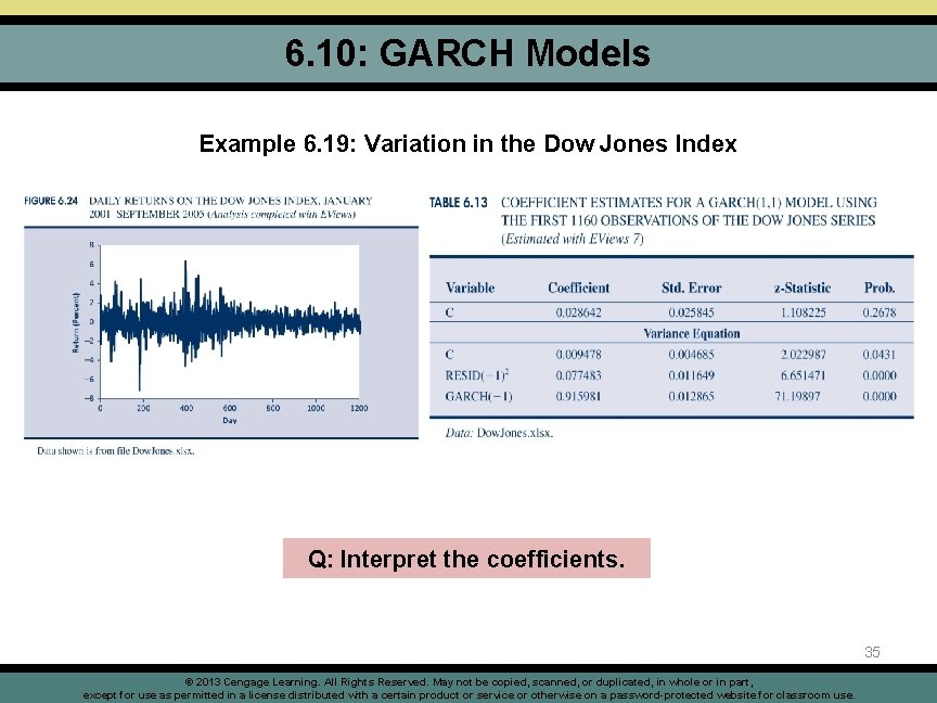
6. 10: GARCH Models • Generalized Autoregressive Conditional Heteroscedastic [GARCH] models provide descriptions of how the error variance evolves over time. • The most commonly used model is the GARCH(1, 1) scheme: • • denotes the variance at time t and error at time t-1. is the squared are parameters subject to the conditions: 34 © 2013 Cengage Learning. All Rights Reserved. May not be copied, scanned, or duplicated, in whole or in part, except for use as permitted in a license distributed with a certain product or service or otherwise on a password-protected website for classroom use.

6. 10: GARCH Models Example 6. 19: Variation in the Dow Jones Index Q: Interpret the coefficients. 35 © 2013 Cengage Learning. All Rights Reserved. May not be copied, scanned, or duplicated, in whole or in part, except for use as permitted in a license distributed with a certain product or service or otherwise on a password-protected website for classroom use.

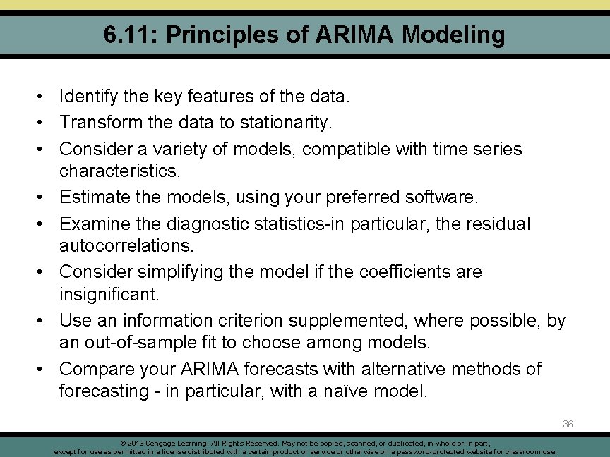
6. 11: Principles of ARIMA Modeling • Identify the key features of the data. • Transform the data to stationarity. • Consider a variety of models, compatible with time series characteristics. • Estimate the models, using your preferred software. • Examine the diagnostic statistics-in particular, the residual autocorrelations. • Consider simplifying the model if the coefficients are insignificant. • Use an information criterion supplemented, where possible, by an out-of-sample fit to choose among models. • Compare your ARIMA forecasts with alternative methods of forecasting - in particular, with a naïve model. 36 © 2013 Cengage Learning. All Rights Reserved. May not be copied, scanned, or duplicated, in whole or in part, except for use as permitted in a license distributed with a certain product or service or otherwise on a password-protected website for classroom use.

6. 11. 2: GARCH Models • Start with a constant variance model, and then examine the autocorrelation structure of the squared residuals, using the methods of this chapter. • The GARCH(1, 1) model will suffice for most purposes. • Remember KISS (Keep It Simple, Statistician)! 37 © 2013 Cengage Learning. All Rights Reserved. May not be copied, scanned, or duplicated, in whole or in part, except for use as permitted in a license distributed with a certain product or service or otherwise on a password-protected website for classroom use.

Take-Aways • The Box-Jenkins or ARIMA approach provides a framework for model selection, estimation and forecasting. • The ACF and PACF are the primary tools for model selection and they are also useful as diagnostic devices. • ARIMA models require the time series to be stationary or to be transformed to stationarity. Typically business series will require differencing and/or transformations to achieve this condition. • There is a general equivalence between linear state-space models and ARIMA models. However, the actual models selected in an application may well differ. • GARCH models provide for changing variances to complement the changes in the mean level. 38 © 2013 Cengage Learning. All Rights Reserved. May not be copied, scanned, or duplicated, in whole or in part, except for use as permitted in a license distributed with a certain product or service or otherwise on a password-protected website for classroom use.