14 GoodnessofFit Tests and Categorical Data Analysis Copyright

14 Goodness-of-Fit Tests and Categorical Data Analysis Copyright © Cengage Learning. All rights reserved.

14. 2 Goodness-of-Fit Tests for Composite Hypotheses Copyright © Cengage Learning. All rights reserved.

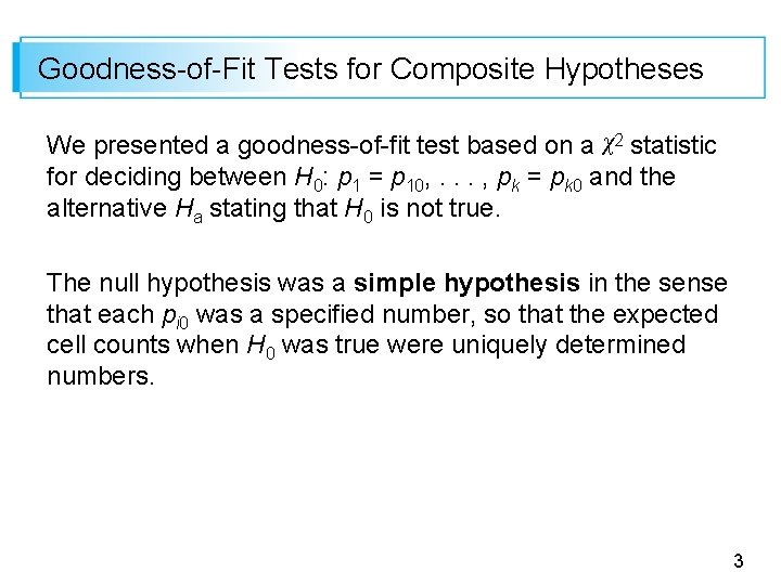
Goodness-of-Fit Tests for Composite Hypotheses We presented a goodness-of-fit test based on a χ2 statistic for deciding between H 0: p 1 = p 10, . . . , pk = pk 0 and the alternative Ha stating that H 0 is not true. The null hypothesis was a simple hypothesis in the sense that each pi 0 was a specified number, so that the expected cell counts when H 0 was true were uniquely determined numbers. 3

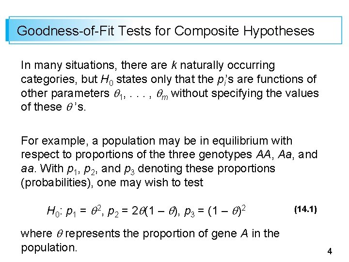
Goodness-of-Fit Tests for Composite Hypotheses In many situations, there are k naturally occurring categories, but H 0 states only that the pi’s are functions of other parameters 1, . . . , m without specifying the values of these ’s. For example, a population may be in equilibrium with respect to proportions of the three genotypes AA, Aa, and aa. With p 1, p 2, and p 3 denoting these proportions (probabilities), one may wish to test H 0: p 1 = 2, p 2 = 2 (1 – ), p 3 = (1 – )2 where represents the proportion of gene A in the population. (14. 1) 4

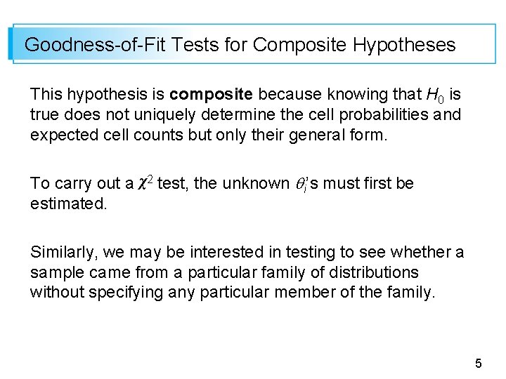
Goodness-of-Fit Tests for Composite Hypotheses This hypothesis is composite because knowing that H 0 is true does not uniquely determine the cell probabilities and expected cell counts but only their general form. To carry out a χ2 test, the unknown i’s must first be estimated. Similarly, we may be interested in testing to see whether a sample came from a particular family of distributions without specifying any particular member of the family. 5

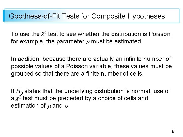
Goodness-of-Fit Tests for Composite Hypotheses To use the χ2 test to see whether the distribution is Poisson, for example, the parameter must be estimated. In addition, because there actually an infinite number of possible values of a Poisson variable, these values must be grouped so that there a finite number of cells. If H 0 states that the underlying distribution is normal, use of a χ2 test must be preceded by a choice of cells and estimation of and . 6

χ2 When Parameters Are Estimated 7

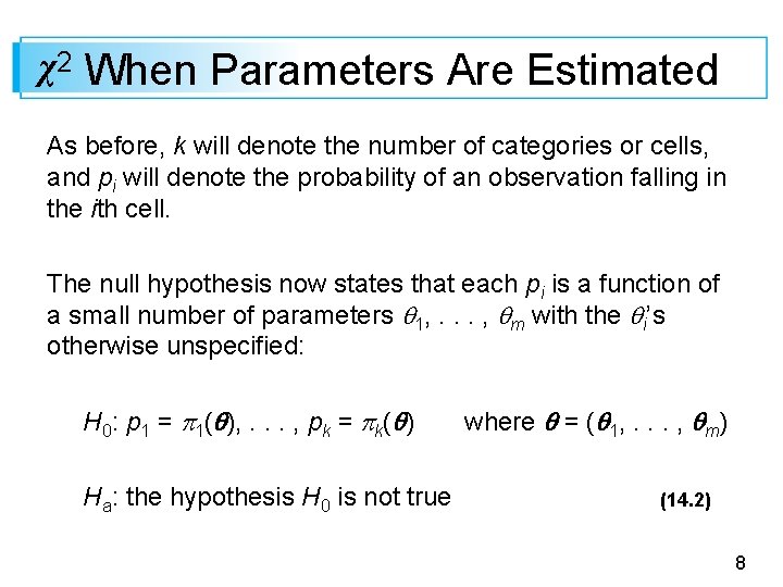
χ2 When Parameters Are Estimated As before, k will denote the number of categories or cells, and pi will denote the probability of an observation falling in the ith cell. The null hypothesis now states that each pi is a function of a small number of parameters 1, . . . , m with the i’s otherwise unspecified: H 0: p 1 = 1( ), . . . , pk = k( ) Ha: the hypothesis H 0 is not true where = ( 1, . . . , m) (14. 2) 8

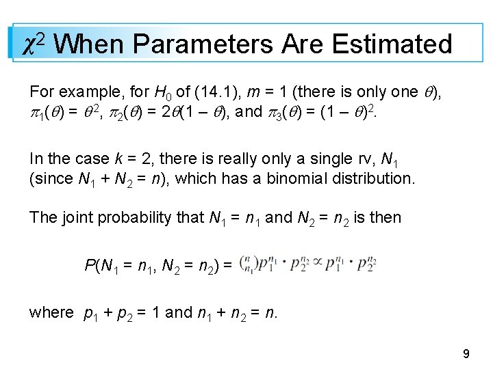
χ2 When Parameters Are Estimated For example, for H 0 of (14. 1), m = 1 (there is only one ), 1( ) = 2, 2( ) = 2 (1 – ), and 3( ) = (1 – )2. In the case k = 2, there is really only a single rv, N 1 (since N 1 + N 2 = n), which has a binomial distribution. The joint probability that N 1 = n 1 and N 2 = n 2 is then P(N 1 = n 1, N 2 = n 2) = where p 1 + p 2 = 1 and n 1 + n 2 = n. 9

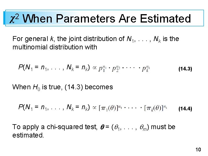
χ2 When Parameters Are Estimated For general k, the joint distribution of N 1, . . . , Nk is the multinomial distribution with P(N 1 = n 1, . . . , Nk = nk) (14. 3) When H 0 is true, (14. 3) becomes P(N 1 = n 1, . . . , Nk = nk) (14. 4) To apply a chi-squared test, = ( 1, . . . , m) must be estimated. 10

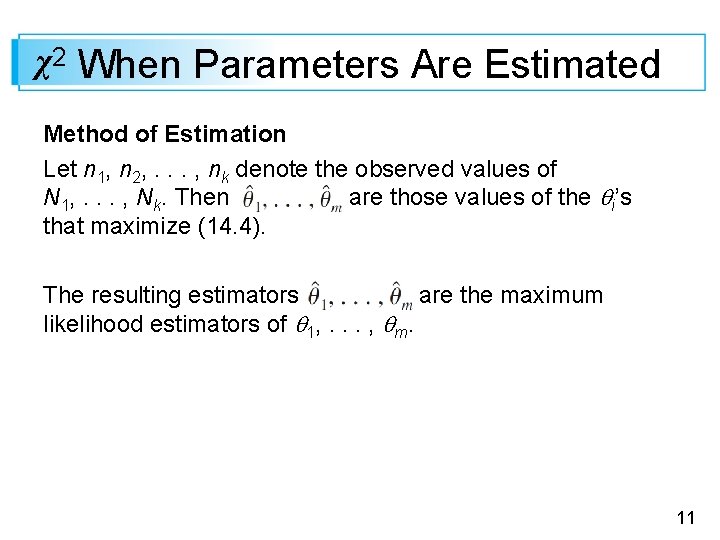
χ2 When Parameters Are Estimated Method of Estimation Let n 1, n 2, . . . , nk denote the observed values of N 1, . . . , Nk. Then are those values of the i’s that maximize (14. 4). The resulting estimators are the maximum likelihood estimators of 1, . . . , m. 11

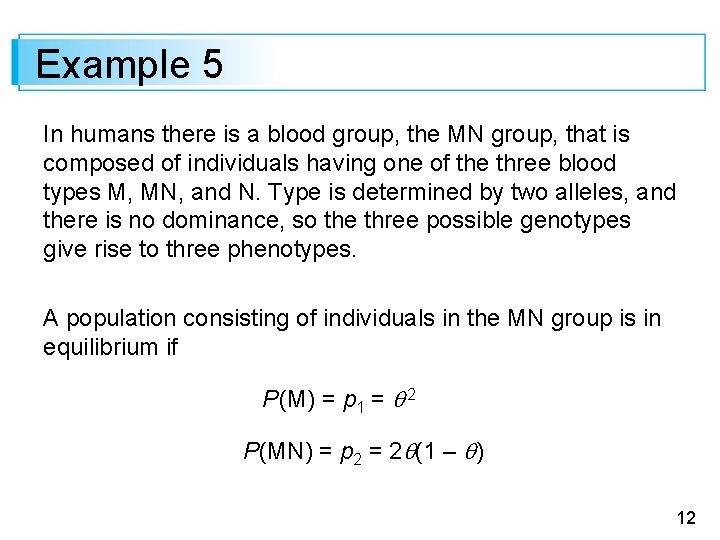
Example 5 In humans there is a blood group, the MN group, that is composed of individuals having one of the three blood types M, MN, and N. Type is determined by two alleles, and there is no dominance, so the three possible genotypes give rise to three phenotypes. A population consisting of individuals in the MN group is in equilibrium if P(M) = p 1 = 2 P(MN) = p 2 = 2 (1 – ) 12

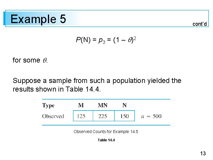
Example 5 cont’d P(N) = p 3 = (1 – )2 for some . Suppose a sample from such a population yielded the results shown in Table 14. 4. Observed Counts for Example 14. 5 Table 14. 4 13

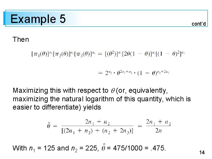
Example 5 cont’d Then Maximizing this with respect to (or, equivalently, maximizing the natural logarithm of this quantity, which is easier to differentiate) yields With n 1 = 125 and n 2 = 225, = 475/1000 =. 475. 14

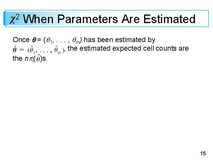
χ2 When Parameters Are Estimated Once = ( 1, . . . , m) has been estimated by , the estimated expected cell counts are the n i( )s. 15

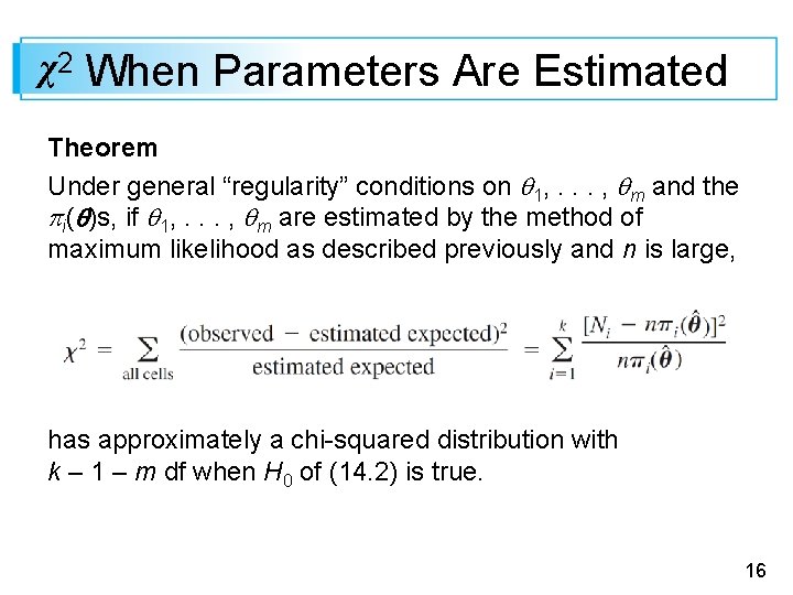
χ2 When Parameters Are Estimated Theorem Under general “regularity” conditions on 1, . . . , m and the i( )s, if 1, . . . , m are estimated by the method of maximum likelihood as described previously and n is large, has approximately a chi-squared distribution with k – 1 – m df when H 0 of (14. 2) is true. 16

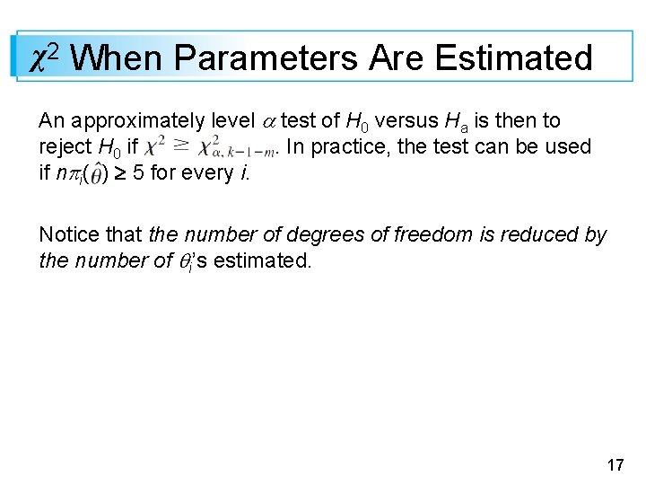
χ2 When Parameters Are Estimated An approximately level test of H 0 versus Ha is then to reject H 0 if. In practice, the test can be used if n i( ) 5 for every i. Notice that the number of degrees of freedom is reduced by the number of i’s estimated. 17

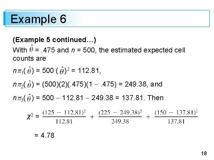
Example 6 (Example 5 continued…) With =. 475 and n = 500, the estimated expected cell counts are n 1( ) = 500 ( )2 = 112. 81, n 2( ) = (500)(2)(. 475)(1 . 475) = 249. 38, and n 3( ) = 500 112. 81 249. 38 = 137. 81. Then χ2 = = 4. 78 18

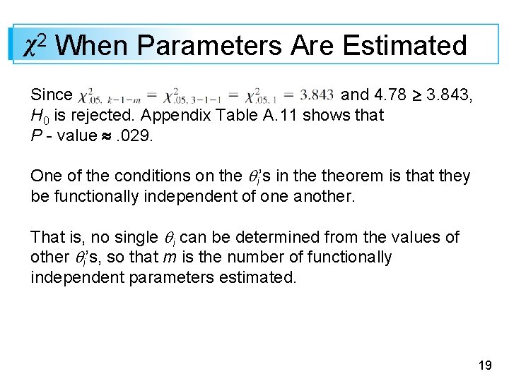
χ2 When Parameters Are Estimated Since and 4. 78 3. 843, H 0 is rejected. Appendix Table A. 11 shows that P - value . 029. One of the conditions on the i’s in theorem is that they be functionally independent of one another. That is, no single i can be determined from the values of other i’s, so that m is the number of functionally independent parameters estimated. 19

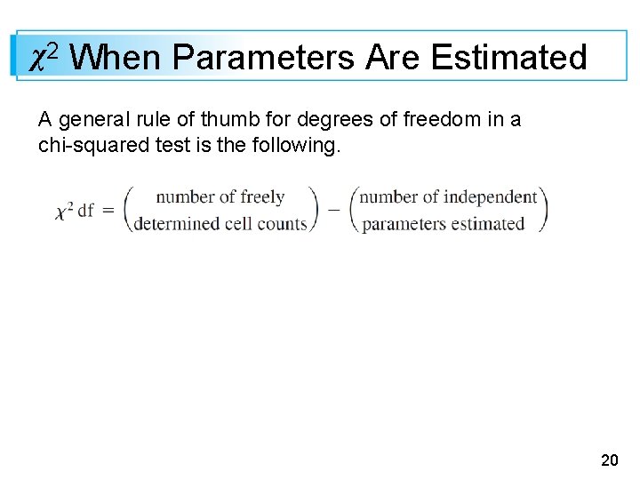
χ2 When Parameters Are Estimated A general rule of thumb for degrees of freedom in a chi-squared test is the following. 20

Goodness of Fit for Discrete Distributions 21

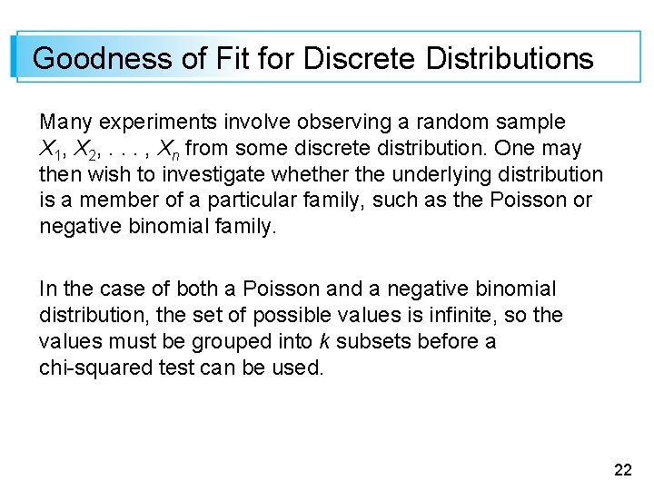
Goodness of Fit for Discrete Distributions Many experiments involve observing a random sample X 1, X 2, . . . , Xn from some discrete distribution. One may then wish to investigate whether the underlying distribution is a member of a particular family, such as the Poisson or negative binomial family. In the case of both a Poisson and a negative binomial distribution, the set of possible values is infinite, so the values must be grouped into k subsets before a chi-squared test can be used. 22

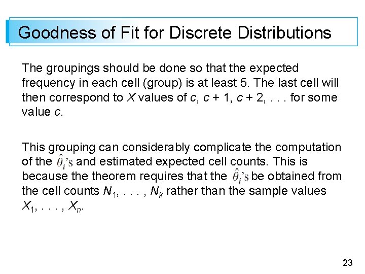
Goodness of Fit for Discrete Distributions The groupings should be done so that the expected frequency in each cell (group) is at least 5. The last cell will then correspond to X values of c, c + 1, c + 2, . . . for some value c. This grouping can considerably complicate the computation of the and estimated expected cell counts. This is because theorem requires that the be obtained from the cell counts N 1, . . . , Nk rather than the sample values X 1, . . . , X n. 23

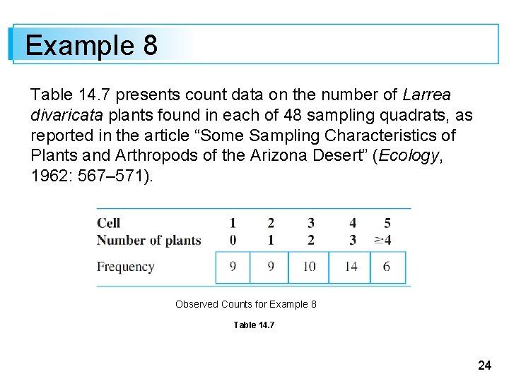
Example 8 Table 14. 7 presents count data on the number of Larrea divaricata plants found in each of 48 sampling quadrats, as reported in the article “Some Sampling Characteristics of Plants and Arthropods of the Arizona Desert” (Ecology, 1962: 567– 571). Observed Counts for Example 8 Table 14. 7 24

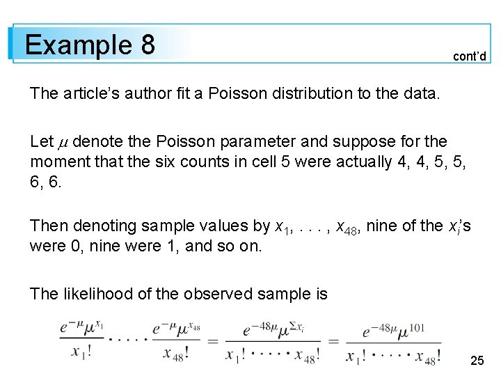
Example 8 cont’d The article’s author fit a Poisson distribution to the data. Let denote the Poisson parameter and suppose for the moment that the six counts in cell 5 were actually 4, 4, 5, 5, 6, 6. Then denoting sample values by x 1, . . . , x 48, nine of the xi’s were 0, nine were 1, and so on. The likelihood of the observed sample is 25

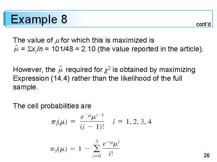
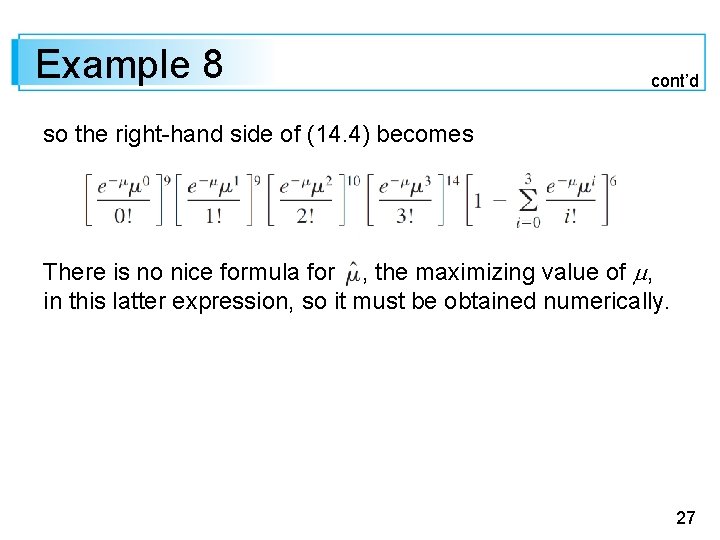
Example 8 cont’d The value of for which this is maximized is = xi /n = 101/48 = 2. 10 (the value reported in the article). However, the required for χ2 is obtained by maximizing Expression (14. 4) rather than the likelihood of the full sample. The cell probabilities are 26

Example 8 cont’d so the right-hand side of (14. 4) becomes There is no nice formula for , the maximizing value of , in this latter expression, so it must be obtained numerically. 27

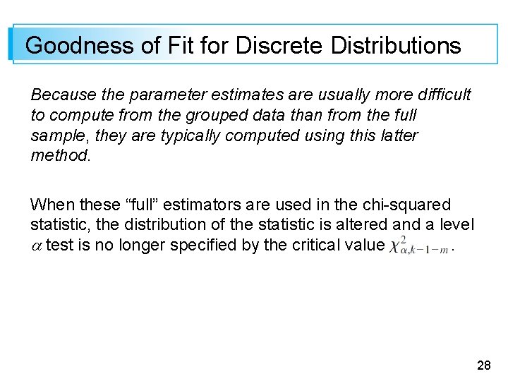
Goodness of Fit for Discrete Distributions Because the parameter estimates are usually more difficult to compute from the grouped data than from the full sample, they are typically computed using this latter method. When these “full” estimators are used in the chi-squared statistic, the distribution of the statistic is altered and a level test is no longer specified by the critical value. 28

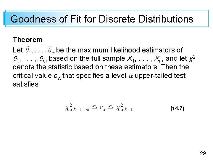
Goodness of Fit for Discrete Distributions Theorem Let be the maximum likelihood estimators of 1, . . . , m based on the full sample X 1, . . . , Xn, and let χ2 denote the statistic based on these estimators. Then the critical value c that specifies a level upper-tailed test satisfies (14. 7) 29

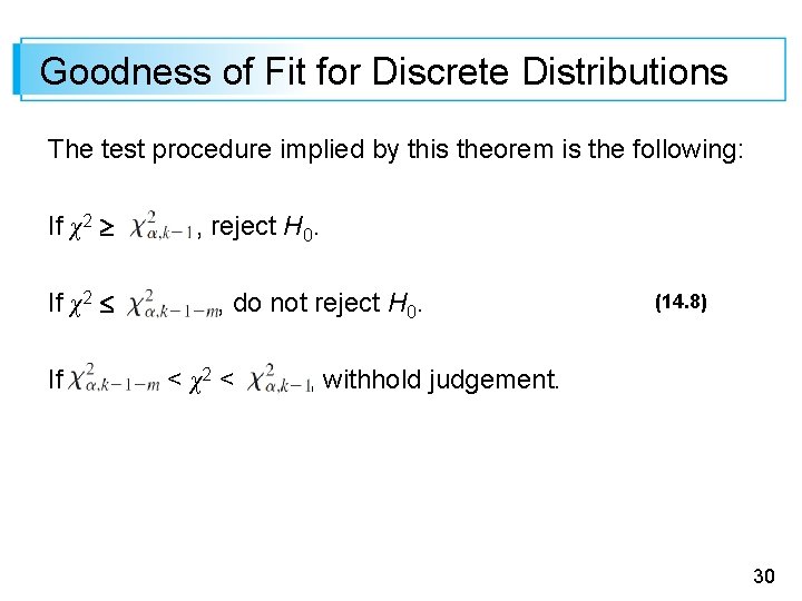
Goodness of Fit for Discrete Distributions The test procedure implied by this theorem is the following: If χ2 If , reject H 0. , do not reject H 0. < χ2 < (14. 8) , withhold judgement. 30

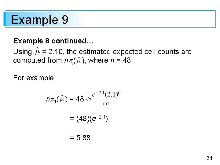
Example 9 Example 8 continued… Using = 2. 10, the estimated expected cell counts are computed from n i( ), where n = 48. For example, n 1( ) = 48 = (48)(e– 2. 1) = 5. 88 31

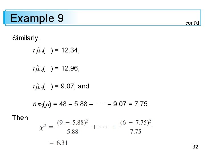
Example 9 cont’d Similarly, n 2( ) = 12. 34, n 3( ) = 12. 96, n 4( ) = 9. 07, and n 5( ) = 48 – 5. 88 – · · · – 9. 07 = 7. 75. Then 32

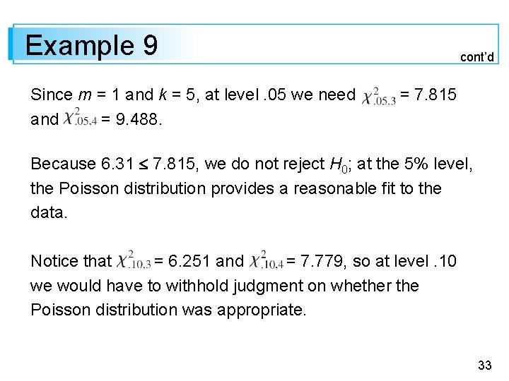
Example 9 Since m = 1 and k = 5, at level. 05 we need and = 9. 488. cont’d = 7. 815 Because 6. 31 7. 815, we do not reject H 0; at the 5% level, the Poisson distribution provides a reasonable fit to the data. Notice that = 6. 251 and = 7. 779, so at level. 10 we would have to withhold judgment on whether the Poisson distribution was appropriate. 33

Goodness of Fit for Continuous Distributions 34

Goodness of Fit for Continuous Distributions The chi-squared test can also be used to test whether the sample comes from a specified family of continuous distributions, such as the exponential family or the normal family. The choice of cells (class intervals) is even more arbitrary in the continuous case than in the discrete case. To ensure that the chi-squared test is valid, the cells should be chosen independently of the sample observations. 35

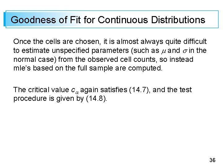
Goodness of Fit for Continuous Distributions Once the cells are chosen, it is almost always quite difficult to estimate unspecified parameters (such as and in the normal case) from the observed cell counts, so instead mle’s based on the full sample are computed. The critical value c again satisfies (14. 7), and the test procedure is given by (14. 8). 36

Example 10 The Institute of Nutrition of Central America and Panama (INCAP) has carried out extensive dietary studies and research projects in Central America. In one study reported in the November 1964 issue of the American Journal of Clinical Nutrition (“The Blood Viscosity of Various Socioeconomic Groups in Guatemala”), serum total cholesterol measurements for a sample of 49 low-income rural Indians were reported as follows (in mg/L): 37

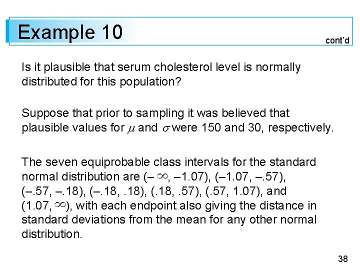
Example 10 cont’d Is it plausible that serum cholesterol level is normally distributed for this population? Suppose that prior to sampling it was believed that plausible values for and were 150 and 30, respectively. The seven equiprobable class intervals for the standard normal distribution are (– , – 1. 07), (– 1. 07, –. 57), (–. 57, –. 18), (–. 18, . 18), (. 18, . 57), (. 57, 1. 07), and (1. 07, ), with each endpoint also giving the distance in standard deviations from the mean for any other normal distribution. 38

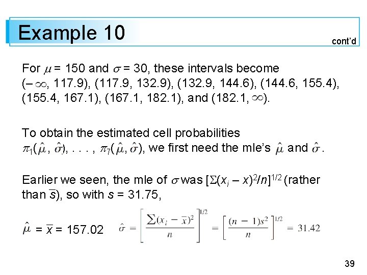
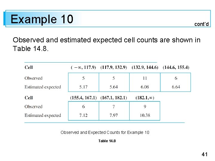
Example 10 cont’d For = 150 and = 30, these intervals become (– , 117. 9), (117. 9, 132. 9), (132. 9, 144. 6), (144. 6, 155. 4), (155. 4, 167. 1), (167. 1, 182. 1), and (182. 1, ). To obtain the estimated cell probabilities 1( , ), . . . , 7( , ), we first need the mle’s and . Earlier we seen, the mle of was [ (xi – x)2/n]1/2 (rather than s), so with s = 31. 75, = x = 157. 02 39

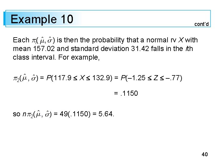
Example 10 cont’d Each i( , ) is then the probability that a normal rv X with mean 157. 02 and standard deviation 31. 42 falls in the ith class interval. For example, 2( , ) = P(117. 9 X 132. 9) = P(– 1. 25 Z –. 77) =. 1150 so n 2( , ) = 49(. 1150) = 5. 64. 40

Example 10 cont’d Observed and estimated expected cell counts are shown in Table 14. 8. Observed and Expected Counts for Example 10 Table 14. 8 41

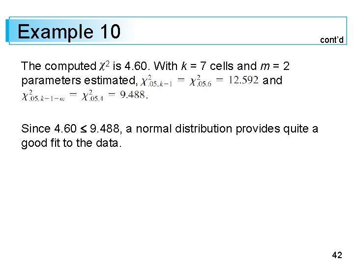
Example 10 cont’d The computed χ2 is 4. 60. With k = 7 cells and m = 2 parameters estimated, and. Since 4. 60 9. 488, a normal distribution provides quite a good fit to the data. 42

A Special Test for Normality 43

A Special Test for Normality As we know that the probability plots are an informal method for assessing the plausibility of any specified population distribution as the one from which the given sample was selected. The straighter the probability plot, the more plausible is the distribution on which the plot is based. A normal probability plot is used for checking whether any member of the normal distribution family is plausible. Let’s denote the sample xi’s when ordered from smallest to largest by 44

A Special Test for Normality Then the plot suggested for checking normality was a plot of the points (x(i), yi), where yi = Φ– 1((i –. 5)/n). A quantitative measure of the extent to which points cluster about a straight line is the sample correlation coefficient r. Consider calculating r for the n pairs (x(1), y 1), . . . , (x(n), yn). The yi’s here are not observed values in a random sample from a y population, so properties of this r are quite different from those described earlier. 45

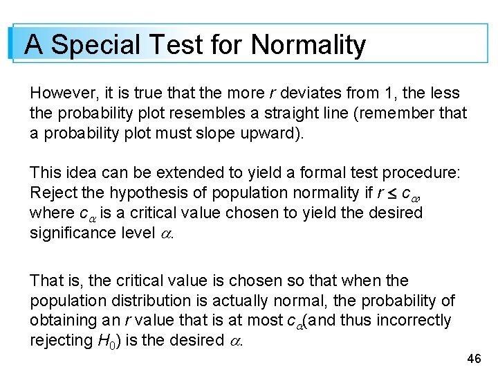
A Special Test for Normality However, it is true that the more r deviates from 1, the less the probability plot resembles a straight line (remember that a probability plot must slope upward). This idea can be extended to yield a formal test procedure: Reject the hypothesis of population normality if r c , where c is a critical value chosen to yield the desired significance level . That is, the critical value is chosen so that when the population distribution is actually normal, the probability of obtaining an r value that is at most c (and thus incorrectly rejecting H 0) is the desired . 46

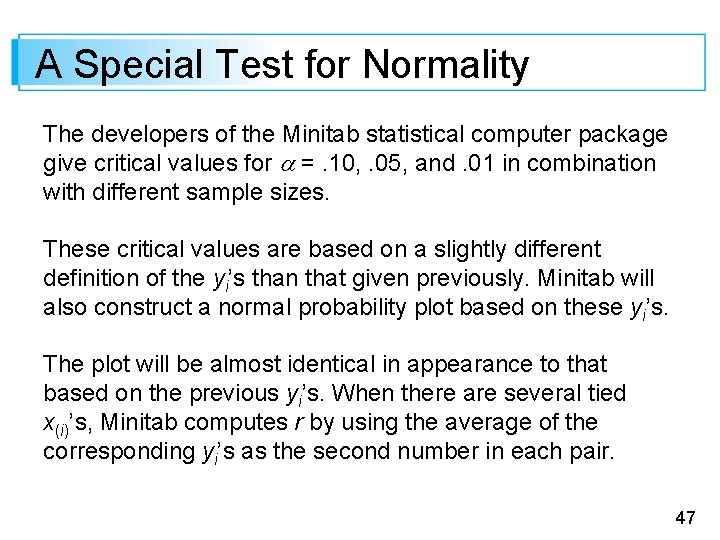
A Special Test for Normality The developers of the Minitab statistical computer package give critical values for =. 10, . 05, and. 01 in combination with different sample sizes. These critical values are based on a slightly different definition of the yi’s than that given previously. Minitab will also construct a normal probability plot based on these yi’s. The plot will be almost identical in appearance to that based on the previous yi’s. When there are several tied x(i)’s, Minitab computes r by using the average of the corresponding yi’s as the second number in each pair. 47

A Special Test for Normality Let yi = Φ– 1[(i –. 375)/(n +. 25)] , and compute the sample correlation coefficient r for the n pairs (x(1), y 1), . . . , (x(n), yn). The Ryan-Joiner test of H 0: the population distribution is normal versus Ha: the population distribution is not normal consists of rejecting H 0 when r c. Critical values c are given in Appendix Table A. 12 for various significance levels and sample sizes n. 48

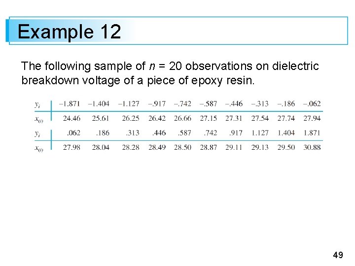
Example 12 The following sample of n = 20 observations on dielectric breakdown voltage of a piece of epoxy resin. 49

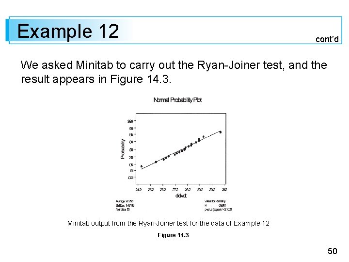
Example 12 cont’d We asked Minitab to carry out the Ryan-Joiner test, and the result appears in Figure 14. 3. Minitab output from the Ryan-Joiner test for the data of Example 12 Figure 14. 3 50

Example 12 cont’d The test statistic value is r =. 9881, and Appendix Table A. 12 gives. 9600 as the critical value that captures lower-tail area. 10 under the r sampling distribution curve when n = 20 and the underlying distribution is actually normal. Since. 9881 >. 9600, the null hypothesis of normality cannot be rejected even for a significance level as large as. 10. 51