14 GoodnessofFit Tests and Categorical Data Analysis Copyright

14 Goodness-of-Fit Tests and Categorical Data Analysis Copyright © Cengage Learning. All rights reserved.

14. 3 Two-Way Contingency Tables Copyright © Cengage Learning. All rights reserved.

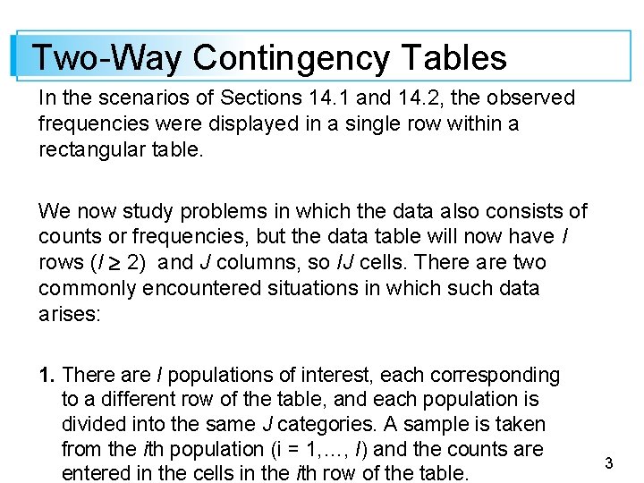
Two-Way Contingency Tables In the scenarios of Sections 14. 1 and 14. 2, the observed frequencies were displayed in a single row within a rectangular table. We now study problems in which the data also consists of counts or frequencies, but the data table will now have I rows (I 2) and J columns, so IJ cells. There are two commonly encountered situations in which such data arises: 1. There are I populations of interest, each corresponding to a different row of the table, and each population is divided into the same J categories. A sample is taken from the ith population (i = 1, …, I) and the counts are entered in the cells in the ith row of the table. 3

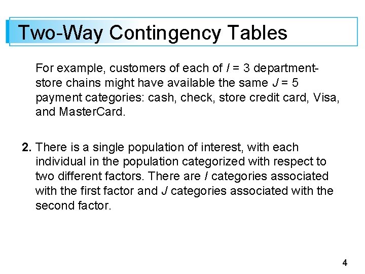
Two-Way Contingency Tables For example, customers of each of I = 3 department- store chains might have available the same J = 5 payment categories: cash, check, store credit card, Visa, and Master. Card. 2. There is a single population of interest, with each individual in the population categorized with respect to two different factors. There are I categories associated with the first factor and J categories associated with the second factor. 4

Two-Way Contingency Tables A single sample is taken, and the number of individuals belonging in both category i of factor 1 and category j of factor 2 is entered in the cell in row i, column j (i = 1, …, I; j = 1, …, J). As an example, customers making a purchase might be classified according to both department in which the purchase was made, with I = 6 departments, and according to method of payment, with J = 5 as in (1) above. 5

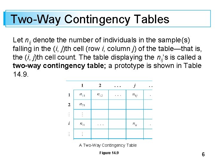
Two-Way Contingency Tables Let nij denote the number of individuals in the sample (s) falling in the (i, j)th cell (row i, column j) of the table—that is, the (i, j)th cell count. The table displaying the nij’s is called a two-way contingency table; a prototype is shown in Table 14. 9. A Two-Way Contingency Table Figure 14. 9 6

Two-Way Contingency Tables In situations of type 1, we want to investigate whether the proportions in the different categories are the same for all populations. The null hypothesis states that the populations are homogeneous with respect to these categories. In type 2 situations, we investigate whether the categories of the two factors occur independently of one another in the population. 7

Testing for Homogeneity 8

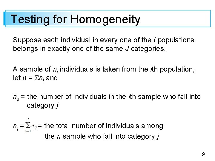
Testing for Homogeneity Suppose each individual in every one of the I populations belongs in exactly one of the same J categories. A sample of ni individuals is taken from the ith population; let n = ni and nij = the number of individuals in the ith sample who fall into category j nj = = the total number of individuals among the n sample who fall into category j 9

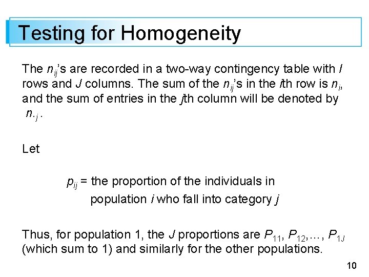
Testing for Homogeneity The nij’s are recorded in a two-way contingency table with I rows and J columns. The sum of the nij’s in the ith row is ni, and the sum of entries in the jth column will be denoted by n. j. Let pij = the proportion of the individuals in population i who fall into category j Thus, for population 1, the J proportions are P 11, P 12, …, P 1 J (which sum to 1) and similarly for the other populations. 10

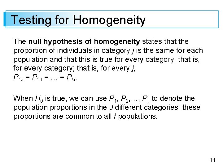
Testing for Homogeneity The null hypothesis of homogeneity states that the proportion of individuals in category j is the same for each population and that this is true for every category; that is, for every j, P 1 J = P 2 J = … = PIJ. When H 0 is true, we can use P 1, P 2, …, PJ to denote the population proportions in the J different categories; these proportions are common to all I populations. 11

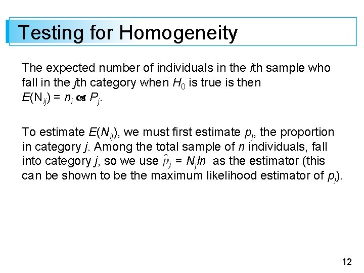
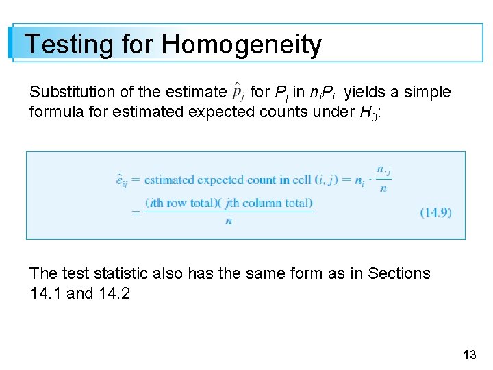
Testing for Homogeneity The expected number of individuals in the ith sample who fall in the jth category when H 0 is true is then E(Nij) = ni Pj. To estimate E(Nij), we must first estimate pj, the proportion in category j. Among the total sample of n individuals, fall into category j, so we use = Njln as the estimator (this can be shown to be the maximum likelihood estimator of pj). 12

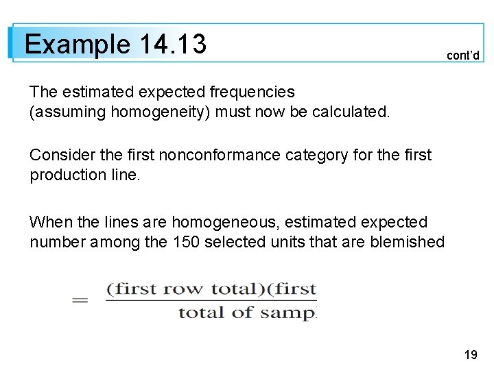
Testing for Homogeneity Substitution of the estimate for Pj in ni. Pj yields a simple formula for estimated expected counts under H 0: The test statistic also has the same form as in Sections 14. 1 and 14. 2 13

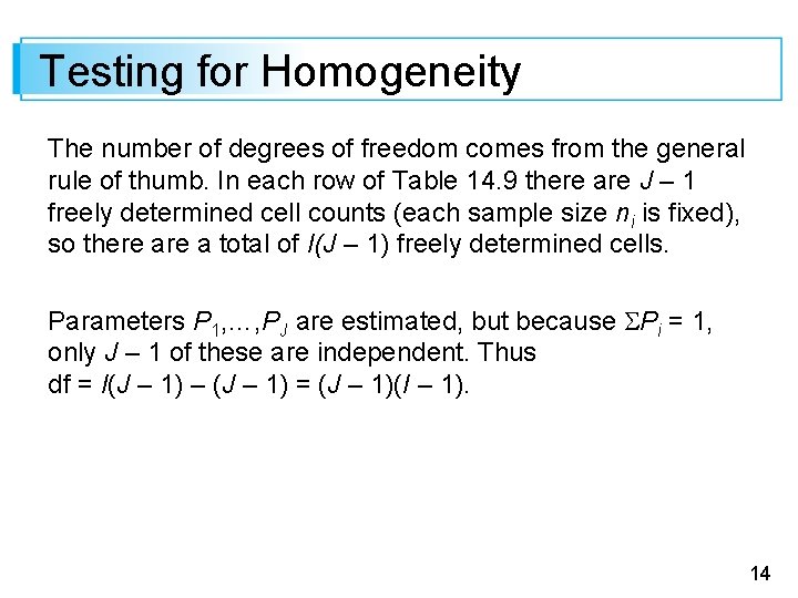
Testing for Homogeneity The number of degrees of freedom comes from the general rule of thumb. In each row of Table 14. 9 there are J – 1 freely determined cell counts (each sample size ni is fixed), so there a total of I(J – 1) freely determined cells. Parameters P 1, …, PJ are estimated, but because Pi = 1, only J – 1 of these are independent. Thus df = I(J – 1) – (J – 1) = (J – 1)(I – 1). 14

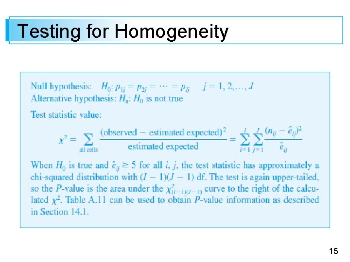
Testing for Homogeneity 15

Example 14. 13 A company packages a particular product in cans of three different sizes, each one using a different production line. Most cans conform to specifications, but a quality control engineer has identified the following reasons for nonconformance: 1. Blemish on can 2. Crack in can 3. Improper pull tab location 4. Pull tab missing 5. Other 16

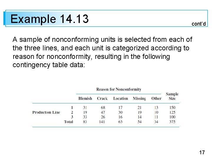
Example 14. 13 cont’d A sample of nonconforming units is selected from each of the three lines, and each unit is categorized according to reason for nonconformity, resulting in the following contingency table data: 17

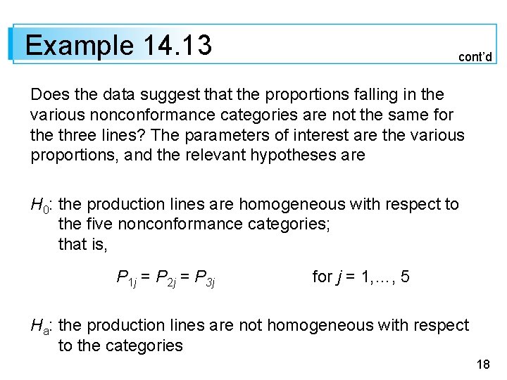
Example 14. 13 cont’d Does the data suggest that the proportions falling in the various nonconformance categories are not the same for the three lines? The parameters of interest are the various proportions, and the relevant hypotheses are H 0: the production lines are homogeneous with respect to the five nonconformance categories; that is, P 1 j = P 2 j = P 3 j for j = 1, …, 5 Ha: the production lines are not homogeneous with respect to the categories 18

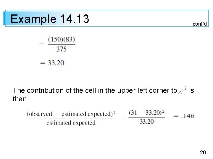
Example 14. 13 cont’d The estimated expected frequencies (assuming homogeneity) must now be calculated. Consider the first nonconformance category for the first production line. When the lines are homogeneous, estimated expected number among the 150 selected units that are blemished 19

Example 14. 13 cont’d The contribution of the cell in the upper-left corner to is then 20

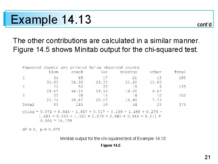
Example 14. 13 cont’d The other contributions are calculated in a similar manner. Figure 14. 5 shows Minitab output for the chi-squared test of Example 14. 13 Figure 14. 5 21

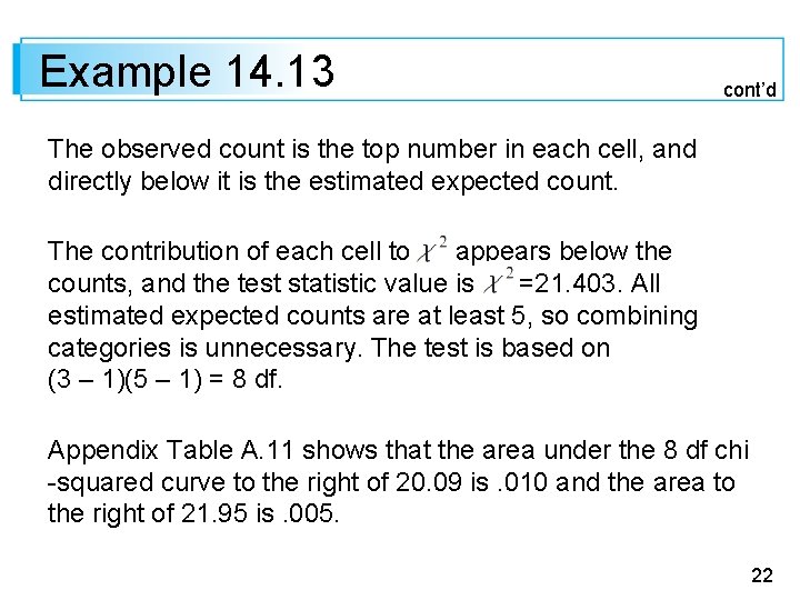
Example 14. 13 cont’d The observed count is the top number in each cell, and directly below it is the estimated expected count. The contribution of each cell to appears below the counts, and the test statistic value is =21. 403. All estimated expected counts are at least 5, so combining categories is unnecessary. The test is based on (3 – 1)(5 – 1) = 8 df. Appendix Table A. 11 shows that the area under the 8 df chi -squared curve to the right of 20. 09 is. 010 and the area to the right of 21. 95 is. 005. 22

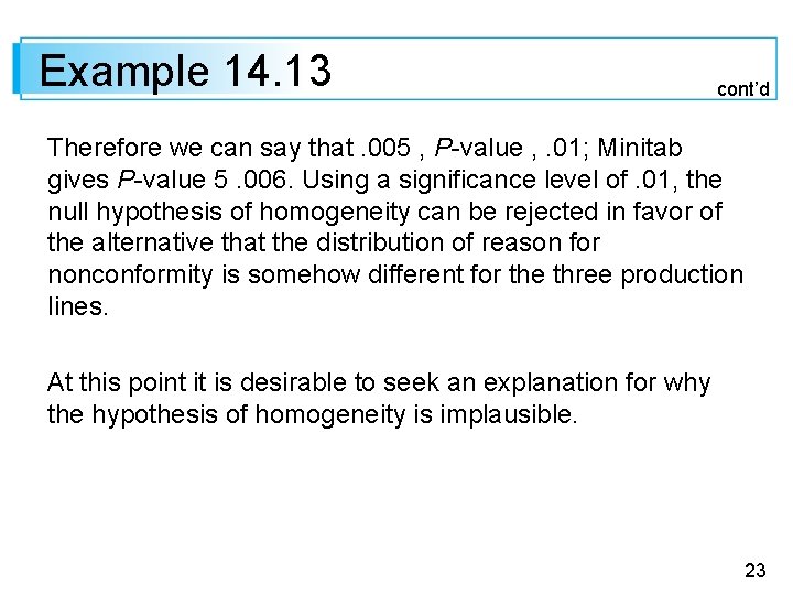
Example 14. 13 cont’d Therefore we can say that. 005 , P-value , . 01; Minitab gives P-value 5. 006. Using a significance level of. 01, the null hypothesis of homogeneity can be rejected in favor of the alternative that the distribution of reason for nonconformity is somehow different for the three production lines. At this point it is desirable to seek an explanation for why the hypothesis of homogeneity is implausible. 23

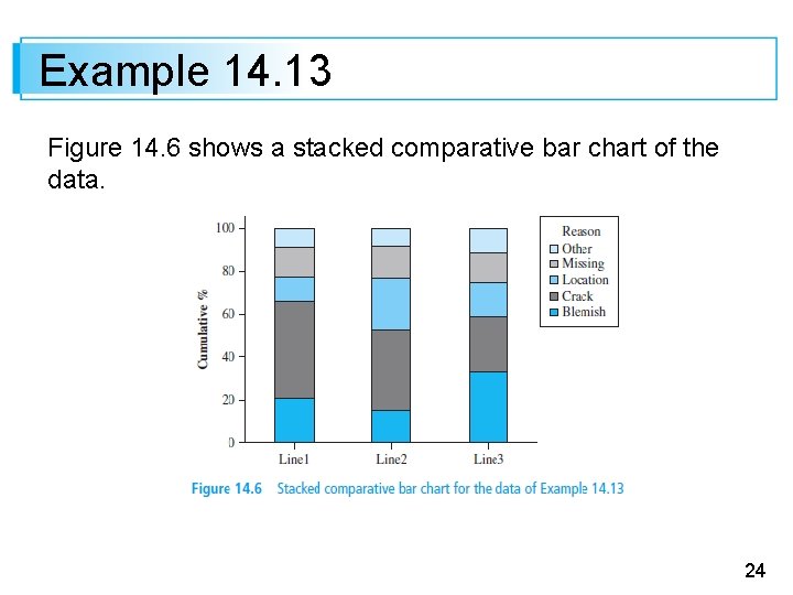
Example 14. 13 Figure 14. 6 shows a stacked comparative bar chart of the data. 24

Example 14. 13 It appears that the three lines are relatively homogenous with respect to the Other and Missing categories but not with respect to the Location, Crack, and Blemish categories. Line 1’s incidence rate of crack nonconformities is much higher than for the other two lines, whereas location nonconformities appear to be more of a problem for line 2 than for the other two lines and blemish nonconformities occur much more frequently for line 3 than for the other two lines. 25

Testing for Independence 26

Testing for Independence (Lack of Association) We focus now on the relationship between two different factors in a single population. Each individual in the population is assumed to belong in exactly one of the I categories associated with the first factor and exactly one of the J categories associated with the second factor. For example, the population of interest might consist of all individuals who regularly watch the national news on television, with the first factor being preferred network (ABC, CBS, NBC, or PBS, so I = 4) and the second factor political philosophy (liberal, moderate, or conservative, giving J = 3). 27

Testing for Independence (Lack of Association) For a sample of n individuals taken from the population, let nij denote the number among the n who fall both in category i of the first factor and category j of the second factor. The nij’s can be displayed in a two-way contingency table with I rows and J columns. In the case of homogeneity for I populations, the row totals were fixed in advance, and only the J column totals were random. 28

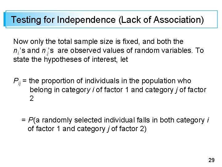
Testing for Independence (Lack of Association) Now only the total sample size is fixed, and both the ni. ’s and n. j’s are observed values of random variables. To state the hypotheses of interest, let Pij = the proportion of individuals in the population who belong in category i of factor 1 and category j of factor 2 = P (a randomly selected individual falls in both category i of factor 1 and category j of factor 2) 29

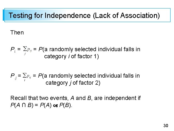
Testing for Independence (Lack of Association) Then Pi. = = P (a randomly selected individual falls in category i of factor 1) P. j = = P (a randomly selected individual falls in category j of factor 2) Recall that two events, A and B, are independent if P(A ∩ B) = P(A) P(B). 30

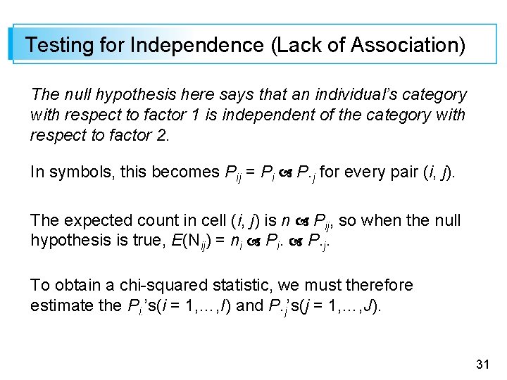
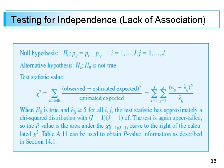
Testing for Independence (Lack of Association) The null hypothesis here says that an individual’s category with respect to factor 1 is independent of the category with respect to factor 2. In symbols, this becomes Pij = Pi P. j for every pair (i, j). The expected count in cell (i, j) is n Pij, so when the null hypothesis is true, E(Nij) = ni Pi. P. j. To obtain a chi-squared statistic, we must therefore estimate the Pi. ’s(i = 1, …, I) and P. j’s(j = 1, …, J). 31

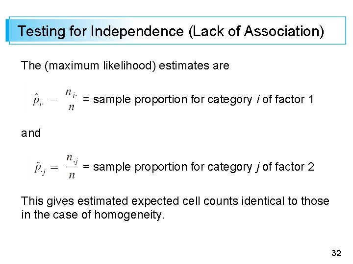
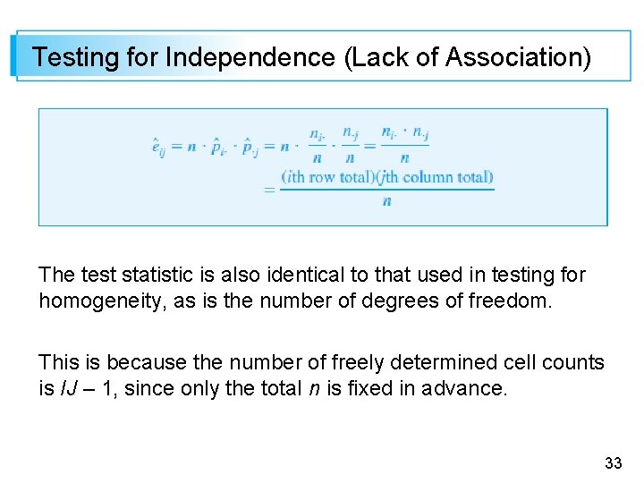
Testing for Independence (Lack of Association) The (maximum likelihood) estimates are = sample proportion for category i of factor 1 and = sample proportion for category j of factor 2 This gives estimated expected cell counts identical to those in the case of homogeneity. 32

Testing for Independence (Lack of Association) The test statistic is also identical to that used in testing for homogeneity, as is the number of degrees of freedom. This is because the number of freely determined cell counts is IJ – 1, since only the total n is fixed in advance. 33

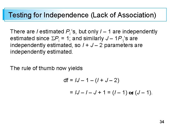
Testing for Independence (Lack of Association) There are I estimated Pi. ’s, but only I – 1 are independently estimated since Pi. = 1; and similarly J – 1 P. j’s are independently estimated, so I + J – 2 parameters are independently estimated. The rule of thumb now yields df = IJ – 1 – (I + J – 2) = IJ – I – J + 1 = (I – 1) (J – 1). 34

Testing for Independence (Lack of Association) 35

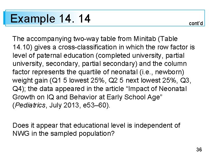
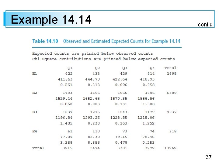
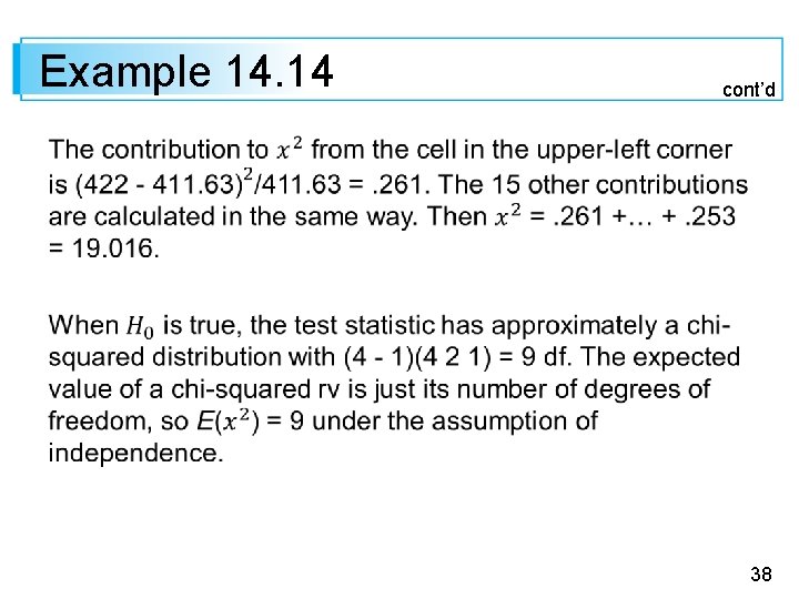
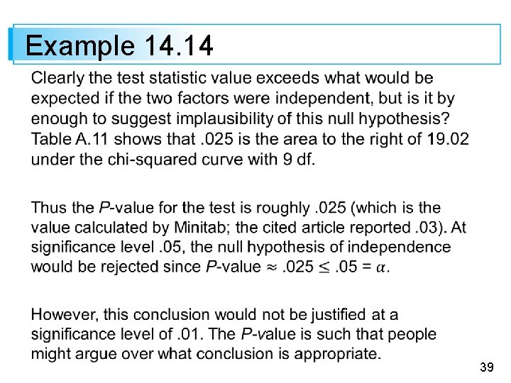
Example 14. 14 cont’d The accompanying two-way table from Minitab (Table 14. 10) gives a cross-classification in which the row factor is level of paternal education (completed university, partial university, secondary, partial secondary) and the column factor represents the quartile of neonatal (i. e. , newborn) weight gain (Q 1 5 lowest 25%, Q 2 5 next lowest 25%, Q 3, Q 4); the data appeared in the article “Impact of Neonatal Growth on IQ and Behavior at Early School Age” (Pediatrics, July 2013, e 53– 60). Does it appear that educational level is independent of NWG in the sampled population? 36

Example 14. 14 cont’d 37

Example 14. 14 cont’d 38

Example 14. 14 39

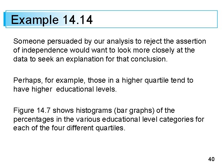
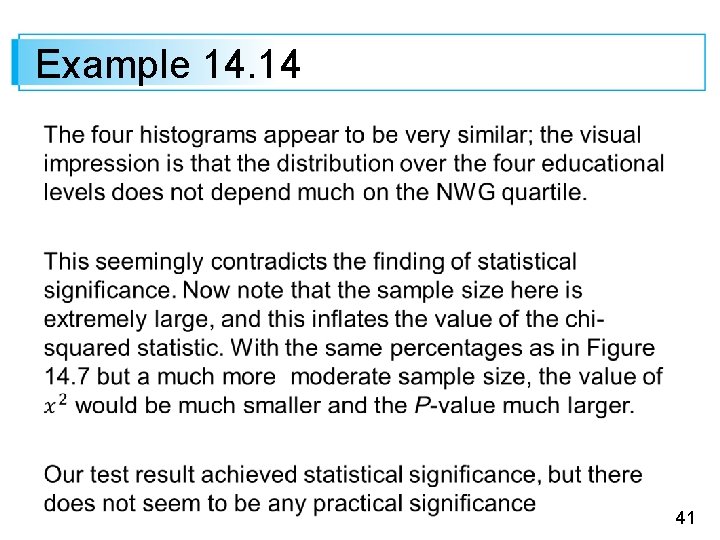
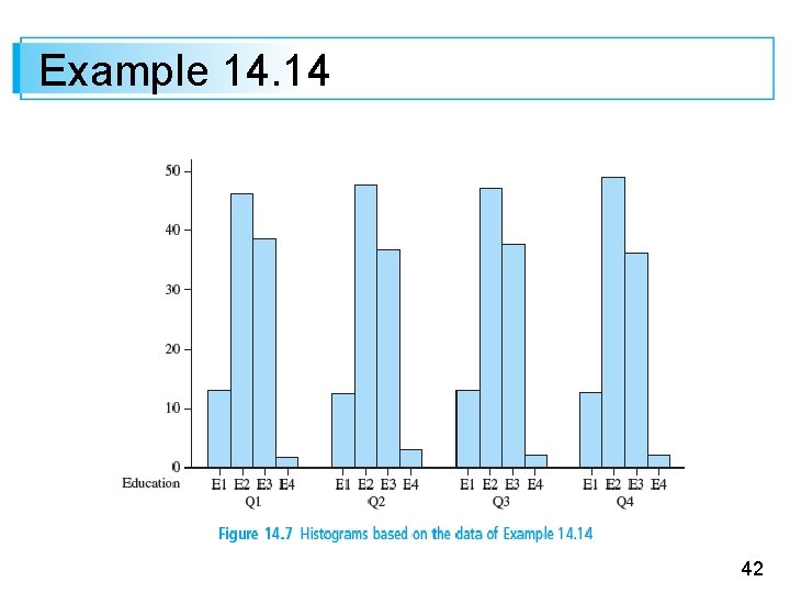
Example 14. 14 Someone persuaded by our analysis to reject the assertion of independence would want to look more closely at the data to seek an explanation for that conclusion. Perhaps, for example, those in a higher quartile tend to have higher educational levels. Figure 14. 7 shows histograms (bar graphs) of the percentages in the various educational level categories for each of the four different quartiles. 40

Example 14. 14 41

Example 14. 14 42

Testing for Independence (Lack of Association) Models and methods for analyzing data in which each individual is categorized with respect to three or more factors (multidimensional contingency tables) are discussed in several of the chapter references. 43