1 Fundamentals Copyright Cengage Learning All rights reserved

1 Fundamentals Copyright © Cengage Learning. All rights reserved.

1. 9 The Coordinate Plane; Graphs of Equations; Circles Copyright © Cengage Learning. All rights reserved.

Objectives ■ The Coordinate Plane ■ The Distance and Midpoint Formulas ■ Graphs of Equations in Two Variables ■ Intercepts ■ Circles ■ Symmetry 3

The Coordinate Plane 4

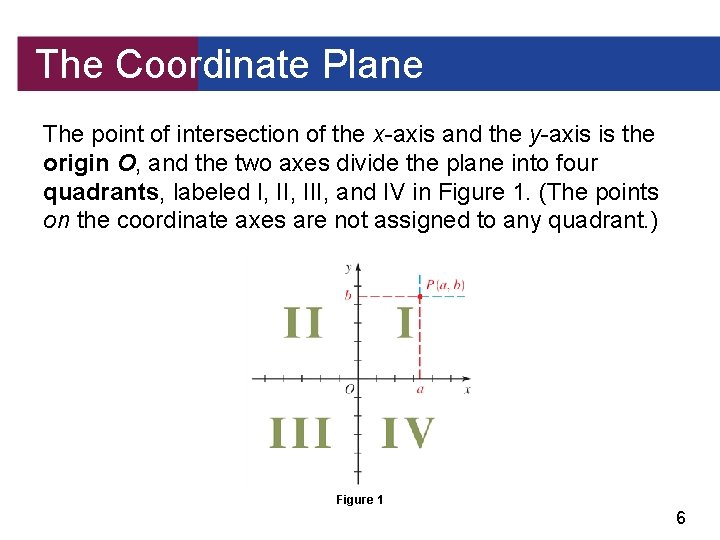
The Coordinate Plane Just as points on a line can be identified with real numbers to form the coordinate line, points in a plane can be identified with ordered pairs of numbers to form the coordinate plane or Cartesian plane. To do this, we draw two perpendicular real lines that intersect at 0 on each line. Usually, one line is horizontal with positive direction to the right and is called the x-axis; the other line is vertical with positive direction upward and is called the y-axis. 5

The Coordinate Plane The point of intersection of the x-axis and the y-axis is the origin O, and the two axes divide the plane into four quadrants, labeled I, III, and IV in Figure 1. (The points on the coordinate axes are not assigned to any quadrant. ) Figure 1 6

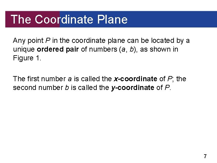
The Coordinate Plane Any point P in the coordinate plane can be located by a unique ordered pair of numbers (a, b), as shown in Figure 1. The first number a is called the x-coordinate of P; the second number b is called the y-coordinate of P. 7

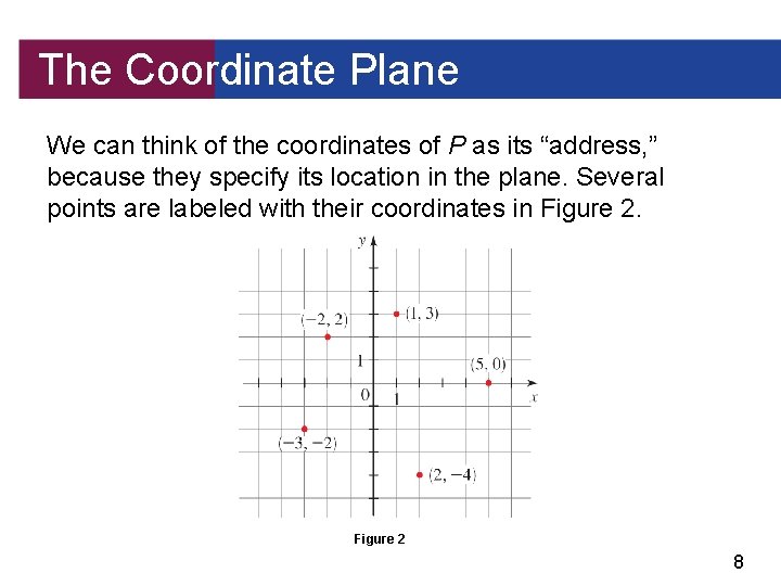
The Coordinate Plane We can think of the coordinates of P as its “address, ” because they specify its location in the plane. Several points are labeled with their coordinates in Figure 2 8

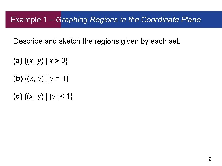
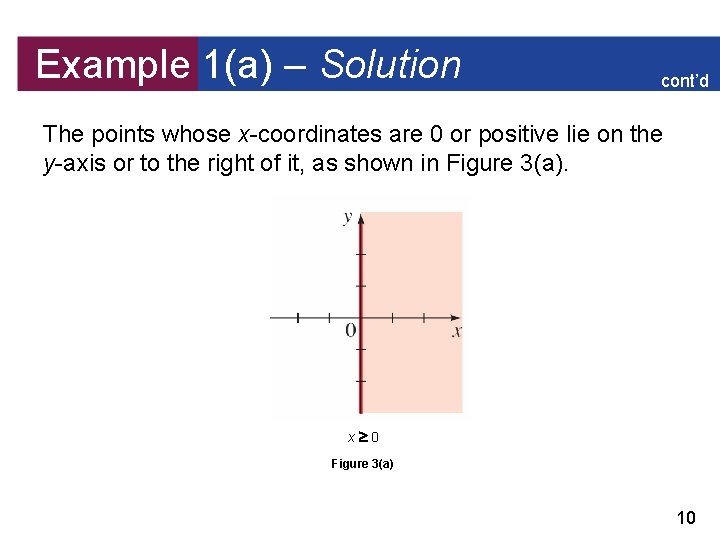
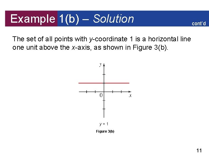
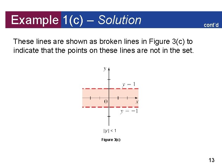
Example 1 – Graphing Regions in the Coordinate Plane Describe and sketch the regions given by each set. (a) {(x, y) | x 0} (b) {(x, y) | y = 1} (c) {(x, y) | | y | < 1} 9

Example 1(a) – Solution cont’d The points whose x-coordinates are 0 or positive lie on the y-axis or to the right of it, as shown in Figure 3(a). x 0 Figure 3(a) 10

Example 1(b) – Solution cont’d The set of all points with y-coordinate 1 is a horizontal line one unit above the x-axis, as shown in Figure 3(b). y=1 Figure 3(b) 11

Example 1(c) – Solution cont’d We know that |y| < 1 if and only if – 1 < y < 1 So the given region consists of those points in the plane whose y-coordinates lie between – 1 and 1. Thus the region consists of all points that lie between (but not on) the horizontal lines y = 1 and y = – 1. 12

Example 1(c) – Solution cont’d These lines are shown as broken lines in Figure 3(c) to indicate that the points on these lines are not in the set. |y| < 1 Figure 3(c) 13

The Distance and Midpoint Formulas 14

The Distance and Midpoint Formulas We now find a formula for the distance d(A, B) between two points A(x 1, y 1) and B(x 2, y 2) in the plane. We know that the distance between points a and b on a number line is d(a, b) = | b – a |. 15

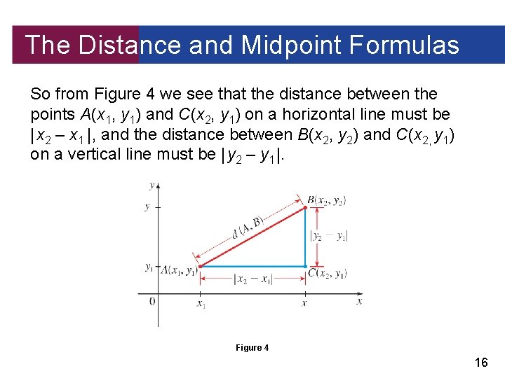
The Distance and Midpoint Formulas So from Figure 4 we see that the distance between the points A(x 1, y 1) and C(x 2, y 1) on a horizontal line must be | x 2 – x 1 |, and the distance between B(x 2, y 2) and C(x 2, y 1) on a vertical line must be | y 2 – y 1 |. Figure 4 16

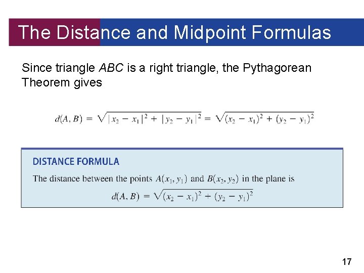
The Distance and Midpoint Formulas Since triangle ABC is a right triangle, the Pythagorean Theorem gives 17

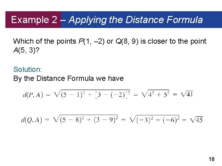
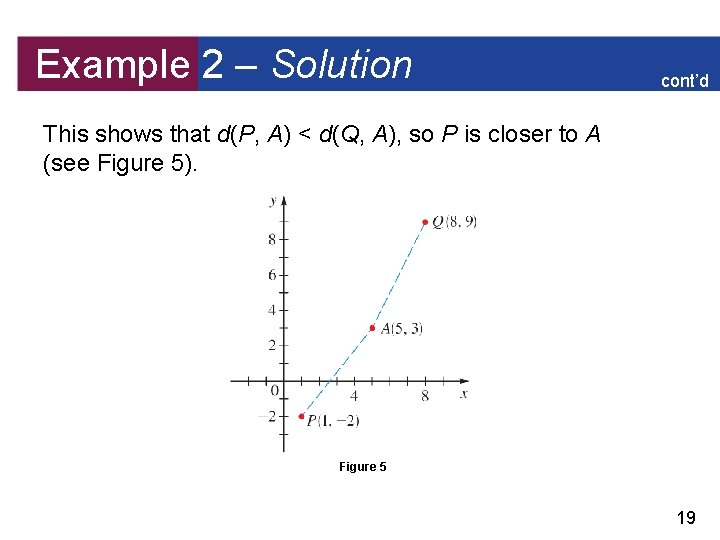
Example 2 – Applying the Distance Formula Which of the points P(1, – 2) or Q(8, 9) is closer to the point A(5, 3)? Solution: By the Distance Formula we have 18

Example 2 – Solution cont’d This shows that d(P, A) < d(Q, A), so P is closer to A (see Figure 5). Figure 5 19

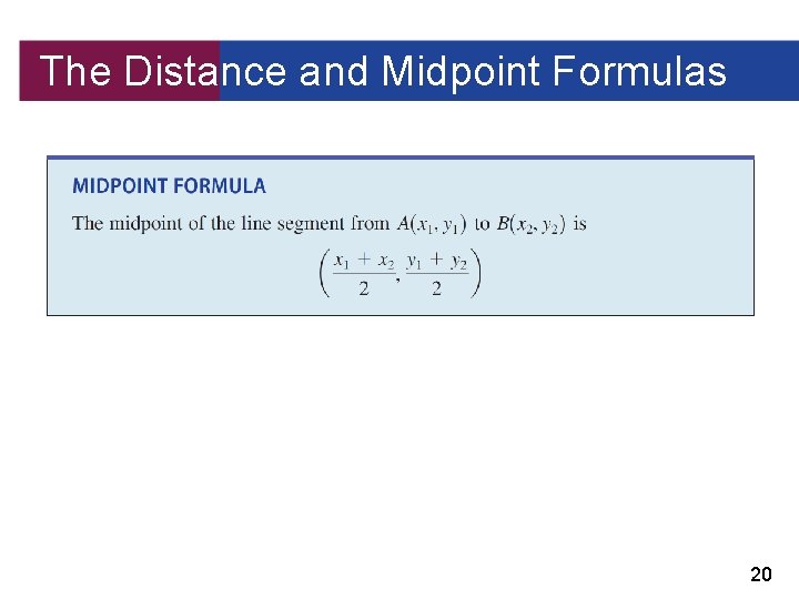
The Distance and Midpoint Formulas 20

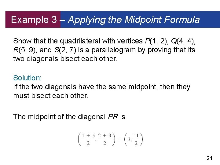
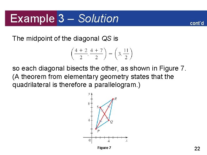
Example 3 – Applying the Midpoint Formula Show that the quadrilateral with vertices P(1, 2), Q(4, 4), R(5, 9), and S(2, 7) is a parallelogram by proving that its two diagonals bisect each other. Solution: If the two diagonals have the same midpoint, then they must bisect each other. The midpoint of the diagonal PR is 21

Example 3 – Solution cont’d The midpoint of the diagonal QS is so each diagonal bisects the other, as shown in Figure 7. (A theorem from elementary geometry states that the quadrilateral is therefore a parallelogram. ) Figure 7 22

Graphs of Equations in Two Variables 23

Graphs of Equations in Two Variables An equation in two variables, such as y = x 2 + 1, expresses a relationship between two quantities. A point (x, y) satisfies the equation if it makes the equation true when the values for x and y are substituted into the equation. For example, the point (3, 10) satisfies the equation y = x 2 + 1 because 10 = 32 + 1, but the point (1, 3) does not, because 3 12 + 1. 24

Graphs of Equations in Two Variables 25

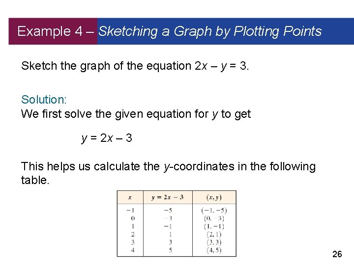
Example 4 – Sketching a Graph by Plotting Points Sketch the graph of the equation 2 x – y = 3. Solution: We first solve the given equation for y to get y = 2 x – 3 This helps us calculate the y-coordinates in the following table. 26

Example 4 – Solution cont’d Of course, there are infinitely many points on the graph, and it is impossible to plot all of them. But the more points we plot, the better we can imagine what the graph represented by the equation looks like. 27

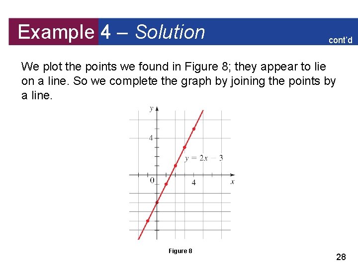
Example 4 – Solution cont’d We plot the points we found in Figure 8; they appear to lie on a line. So we complete the graph by joining the points by a line. Figure 8 28

Intercepts 29

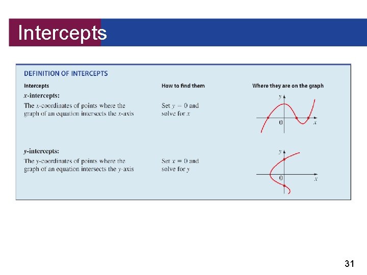
Intercepts The x-coordinates of the points where a graph intersects the x-axis are called the x-intercepts of the graph and are obtained by setting y = 0 in the equation of the graph. The y-coordinates of the points where a graph intersects the y-axis are called the y-intercepts of the graph and are obtained by setting x = 0 in the equation of the graph. 30

Intercepts 31

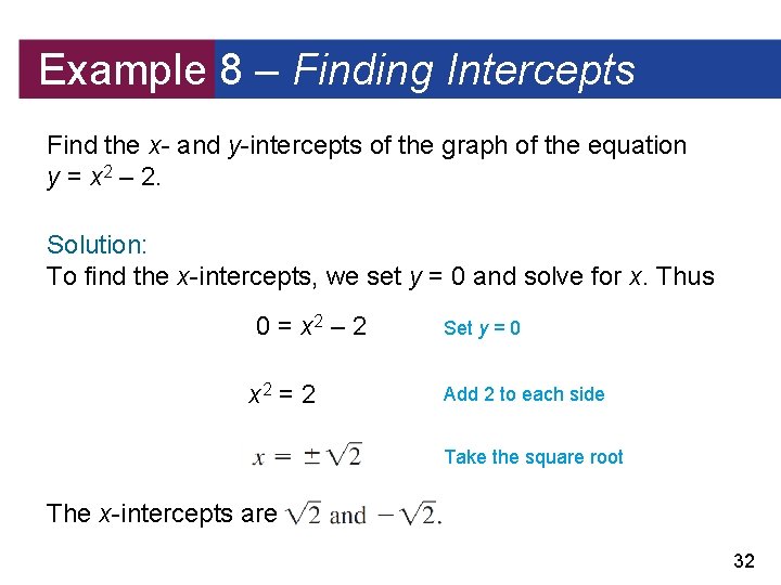
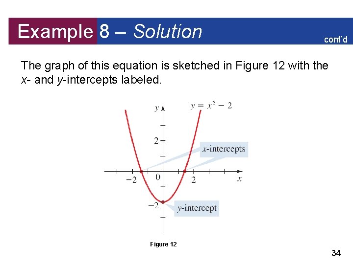
Example 8 – Finding Intercepts Find the x- and y-intercepts of the graph of the equation y = x 2 – 2. Solution: To find the x-intercepts, we set y = 0 and solve for x. Thus 0 = x 2 – 2 x 2 = 2 Set y = 0 Add 2 to each side Take the square root The x-intercepts are 32

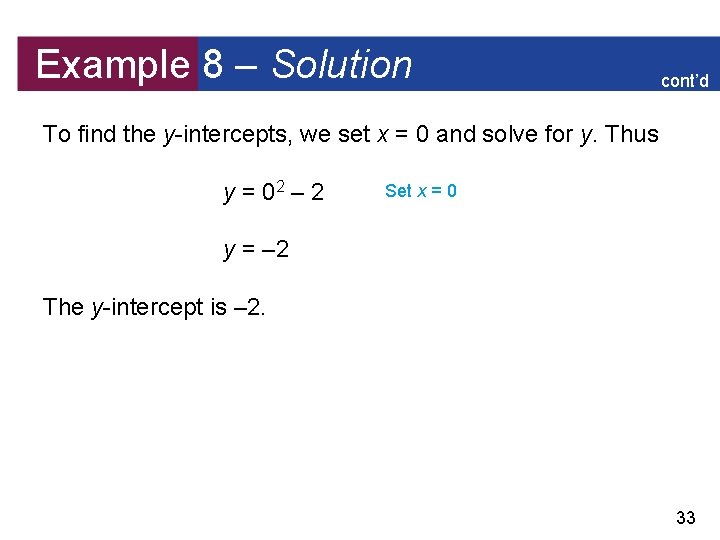
Example 8 – Solution cont’d To find the y-intercepts, we set x = 0 and solve for y. Thus y = 02 – 2 Set x = 0 y = – 2 The y-intercept is – 2. 33

Example 8 – Solution cont’d The graph of this equation is sketched in Figure 12 with the x- and y-intercepts labeled. Figure 12 34

Circles 35

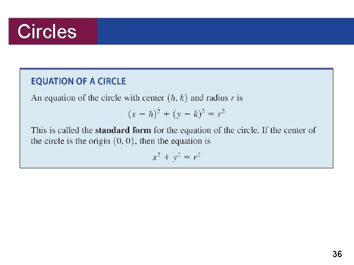
Circles 36

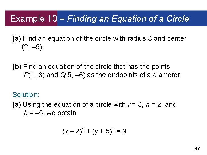
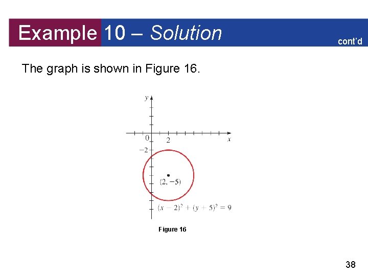
Example 10 – Finding an Equation of a Circle (a) Find an equation of the circle with radius 3 and center (2, – 5). (b) Find an equation of the circle that has the points P(1, 8) and Q(5, – 6) as the endpoints of a diameter. Solution: (a) Using the equation of a circle with r = 3, h = 2, and k = – 5, we obtain (x – 2)2 + (y + 5)2 = 9 37

Example 10 – Solution cont’d The graph is shown in Figure 16 38

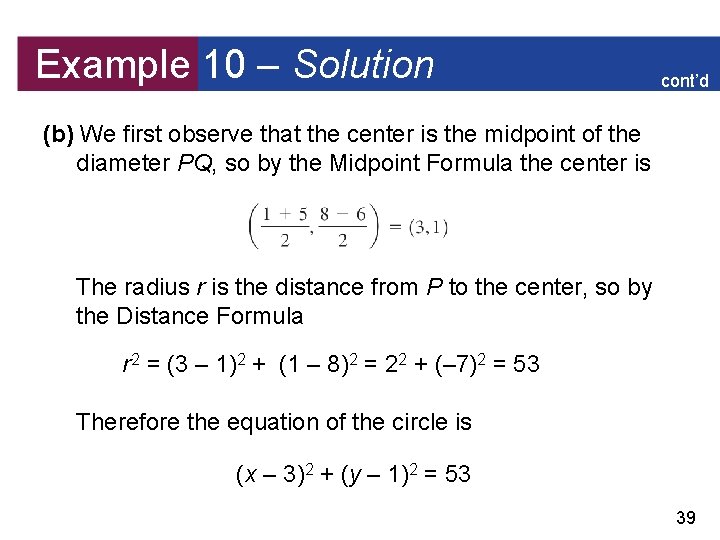
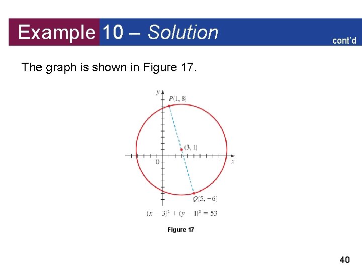
Example 10 – Solution cont’d (b) We first observe that the center is the midpoint of the diameter PQ, so by the Midpoint Formula the center is The radius r is the distance from P to the center, so by the Distance Formula r 2 = (3 – 1)2 + (1 – 8)2 = 22 + (– 7)2 = 53 Therefore the equation of the circle is (x – 3)2 + (y – 1)2 = 53 39

Example 10 – Solution cont’d The graph is shown in Figure 17 40

Symmetry 41

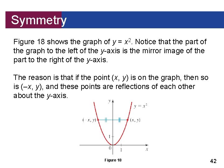
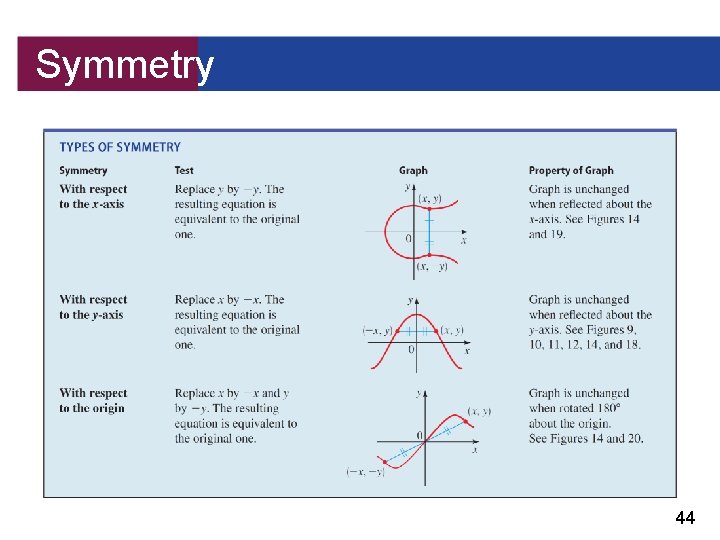
Symmetry Figure 18 shows the graph of y = x 2. Notice that the part of the graph to the left of the y-axis is the mirror image of the part to the right of the y-axis. The reason is that if the point (x, y) is on the graph, then so is (–x, y), and these points are reflections of each other about the y-axis. Figure 18 42

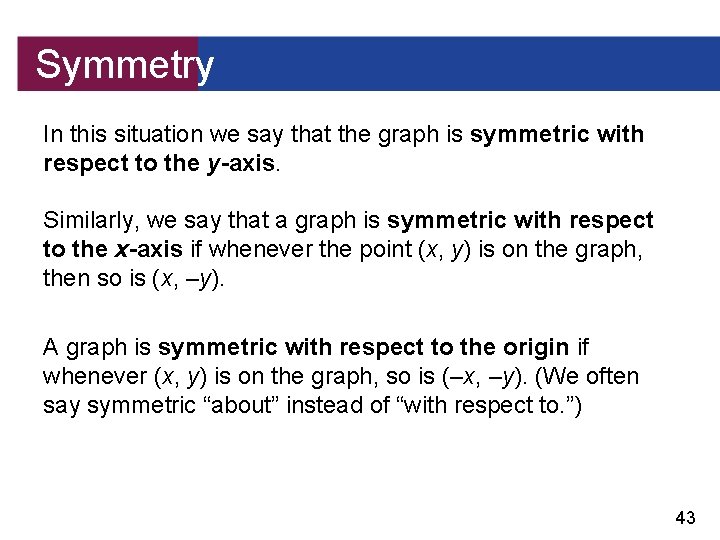
Symmetry In this situation we say that the graph is symmetric with respect to the y-axis. Similarly, we say that a graph is symmetric with respect to the x-axis if whenever the point (x, y) is on the graph, then so is (x, –y). A graph is symmetric with respect to the origin if whenever (x, y) is on the graph, so is (–x, –y). (We often say symmetric “about” instead of “with respect to. ”) 43

Symmetry 44

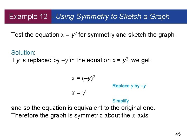
Example 12 – Using Symmetry to Sketch a Graph Test the equation x = y 2 for symmetry and sketch the graph. Solution: If y is replaced by –y in the equation x = y 2, we get x = (–y)2 Replace y by –y x = y 2 Simplify and so the equation is equivalent to the original one. Therefore the graph is symmetric about the x-axis. 45

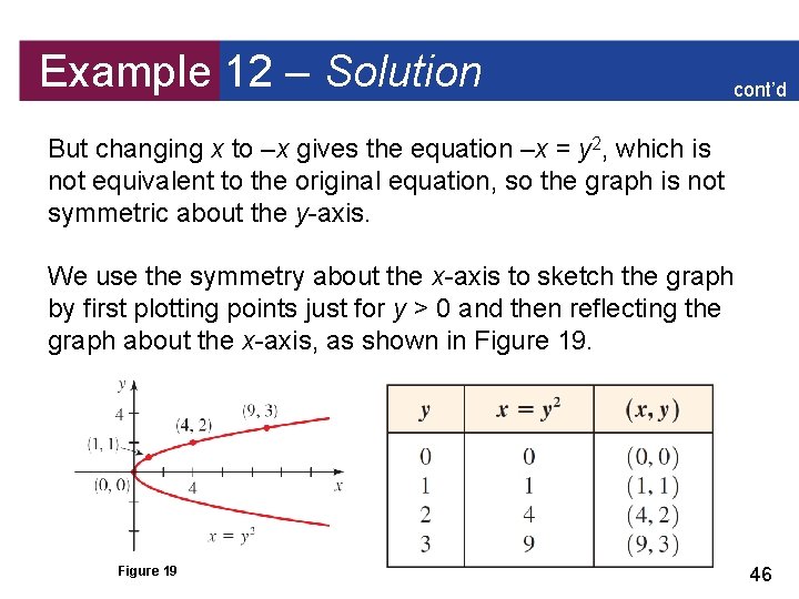
Example 12 – Solution cont’d But changing x to –x gives the equation –x = y 2, which is not equivalent to the original equation, so the graph is not symmetric about the y-axis. We use the symmetry about the x-axis to sketch the graph by first plotting points just for y > 0 and then reflecting the graph about the x-axis, as shown in Figure 19 46