1 Functions and Their Graphs Copyright Cengage Learning

1 Functions and Their Graphs Copyright © Cengage Learning. All rights reserved.

1. 10 Mathematical Modeling with Variation Copyright © Cengage Learning. All rights reserved.

Direct Variation 3

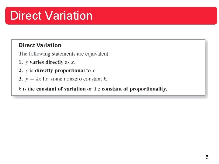
Direct Variation There are two basic types of linear models. The more general model has a y-intercept that is nonzero. y = mx + b, b 0 The simpler model y = kx has a y-intercept that is zero. In the simpler model, y is said to vary directly as x, or to be directly proportional to x. 4

Direct Variation 5

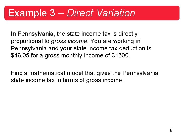
Example 3 – Direct Variation In Pennsylvania, the state income tax is directly proportional to gross income. You are working in Pennsylvania and your state income tax deduction is $46. 05 for a gross monthly income of $1500. Find a mathematical model that gives the Pennsylvania state income tax in terms of gross income. 6

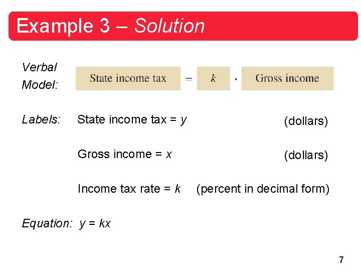
Example 3 – Solution Verbal Model: Labels: State income tax = y (dollars) Gross income = x (dollars) Income tax rate = k (percent in decimal form) Equation: y = kx 7

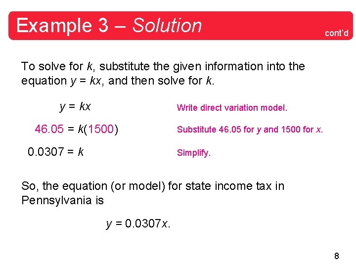
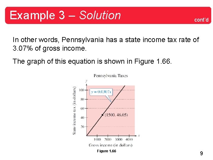
Example 3 – Solution cont’d To solve for k, substitute the given information into the equation y = kx, and then solve for k. y = kx Write direct variation model. 46. 05 = k(1500) 0. 0307 = k Substitute 46. 05 for y and 1500 for x. Simplify. So, the equation (or model) for state income tax in Pennsylvania is y = 0. 0307 x. 8

Example 3 – Solution cont’d In other words, Pennsylvania has a state income tax rate of 3. 07% of gross income. The graph of this equation is shown in Figure 1. 66 9

Direct Variation as an nth Power 10

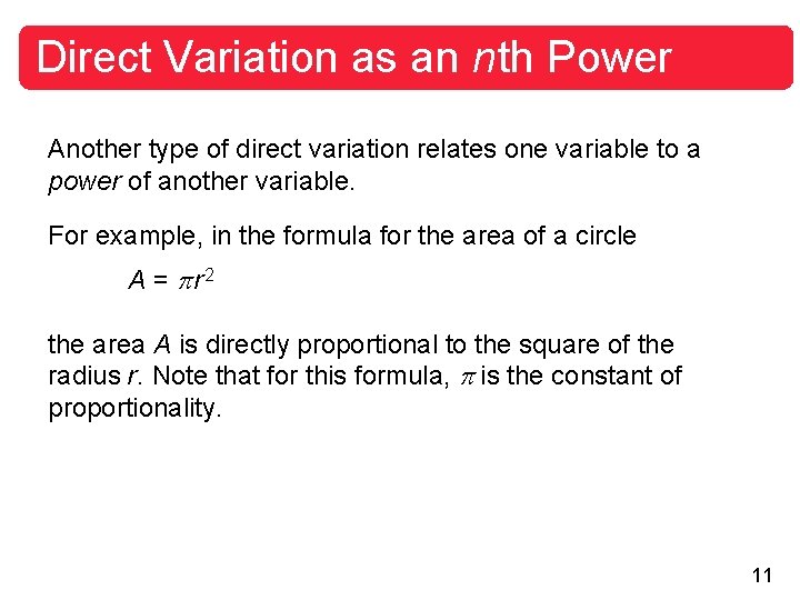
Direct Variation as an nth Power Another type of direct variation relates one variable to a power of another variable. For example, in the formula for the area of a circle A = r 2 the area A is directly proportional to the square of the radius r. Note that for this formula, is the constant of proportionality. 11

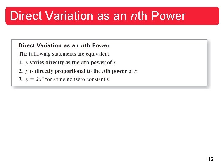
Direct Variation as an nth Power 12

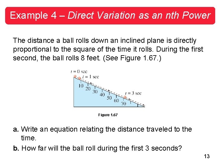
Example 4 – Direct Variation as an nth Power The distance a ball rolls down an inclined plane is directly proportional to the square of the time it rolls. During the first second, the ball rolls 8 feet. (See Figure 1. 67. ) Figure 1. 67 a. Write an equation relating the distance traveled to the time. b. How far will the ball roll during the first 3 seconds? 13

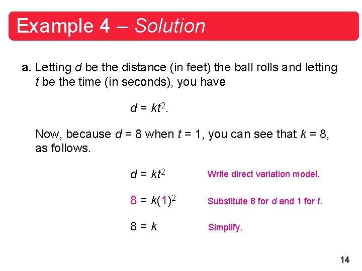
Example 4 – Solution a. Letting d be the distance (in feet) the ball rolls and letting t be the time (in seconds), you have d = kt 2. Now, because d = 8 when t = 1, you can see that k = 8, as follows. d = kt 2 Write direct variation model. 8 = k(1)2 Substitute 8 for d and 1 for t. 8=k Simplify. 14

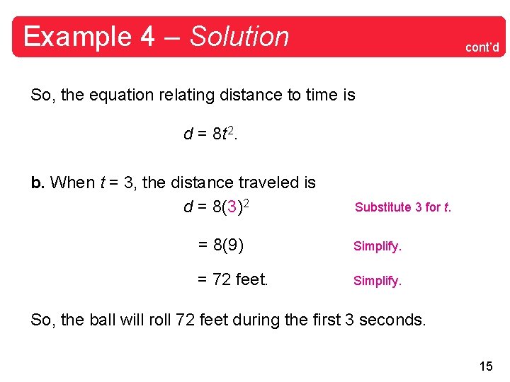
Example 4 – Solution cont’d So, the equation relating distance to time is d = 8 t 2. b. When t = 3, the distance traveled is d = 8(3)2 Substitute 3 for t. = 8(9) Simplify. = 72 feet. Simplify. So, the ball will roll 72 feet during the first 3 seconds. 15

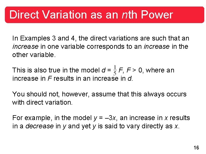
Direct Variation as an nth Power In Examples 3 and 4, the direct variations are such that an increase in one variable corresponds to an increase in the other variable. This is also true in the model d = F, F > 0, where an increase in F results in an increase in d. You should not, however, assume that this always occurs with direct variation. For example, in the model y = – 3 x, an increase in x results in a decrease in y and yet y is said to vary directly as x. 16

Inverse Variation 17

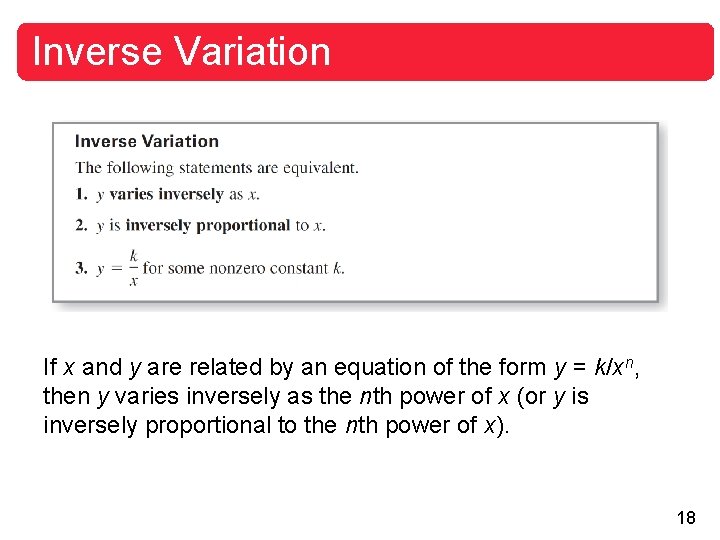
Inverse Variation If x and y are related by an equation of the form y = k/x n, then y varies inversely as the nth power of x (or y is inversely proportional to the nth power of x). [ 18

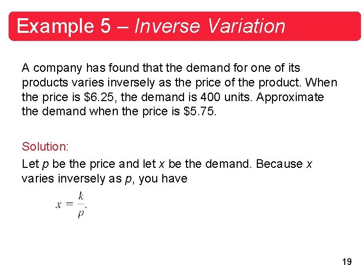
Example 5 – Inverse Variation A company has found that the demand for one of its products varies inversely as the price of the product. When the price is $6. 25, the demand is 400 units. Approximate the demand when the price is $5. 75. Solution: Let p be the price and let x be the demand. Because x varies inversely as p, you have 19

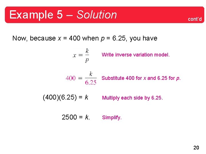
Example 5 – Solution cont’d Now, because x = 400 when p = 6. 25, you have Write inverse variation model. Substitute 400 for x and 6. 25 for p. (400)(6. 25) = k 2500 = k. Multiply each side by 6. 25. Simplify. 20

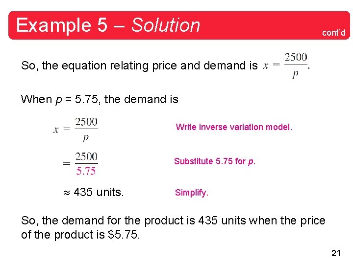
Example 5 – Solution cont’d So, the equation relating price and demand is When p = 5. 75, the demand is Write inverse variation model. Substitute 5. 75 for p. 435 units. Simplify. So, the demand for the product is 435 units when the price of the product is $5. 75. 21

Combined Variation 22

Combined Variation Some applications of variation involve problems with both direct and inverse variations in the same model. These types of models are said to have combined variation. 23

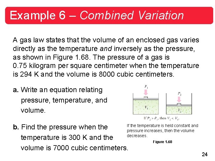
Example 6 – Combined Variation A gas law states that the volume of an enclosed gas varies directly as the temperature and inversely as the pressure, as shown in Figure 1. 68. The pressure of a gas is 0. 75 kilogram per square centimeter when the temperature is 294 K and the volume is 8000 cubic centimeters. a. Write an equation relating pressure, temperature, and volume. If the temperature is held constant and b. Find the pressure when the pressure increases, then the volume decreases. temperature is 300 K and the Figure 1. 68 volume is 7000 cubic centimeters. 24

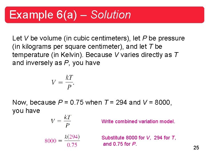
Example 6(a) – Solution Let V be volume (in cubic centimeters), let P be pressure (in kilograms per square centimeter), and let T be temperature (in Kelvin). Because V varies directly as T and inversely as P, you have Now, because P = 0. 75 when T = 294 and V = 8000, you have Write combined variation model. Substitute 8000 for V, 294 for T, and 0. 75 for P. 25

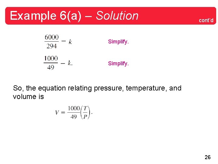
Example 6(a) – Solution cont’d Simplify. So, the equation relating pressure, temperature, and volume is 26

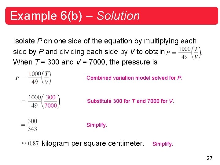
Example 6(b) – Solution Isolate P on one side of the equation by multiplying each side by P and dividing each side by V to obtain When T = 300 and V = 7000, the pressure is Combined variation model solved for P. Substitute 300 for T and 7000 for V. Simplify. kilogram per square centimeter. Simplify. 27

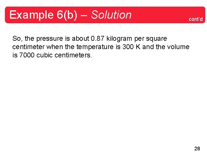
Example 6(b) – Solution cont’d So, the pressure is about 0. 87 kilogram per square centimeter when the temperature is 300 K and the volume is 7000 cubic centimeters. 28

Joint Variation 29

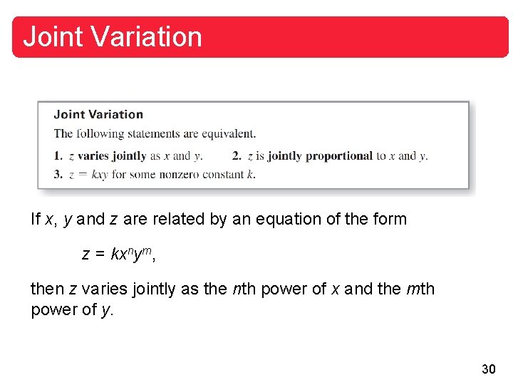
Joint Variation If x, y and z are related by an equation of the form z = kxnym, then z varies jointly as the nth power of x and the mth power of y. 30

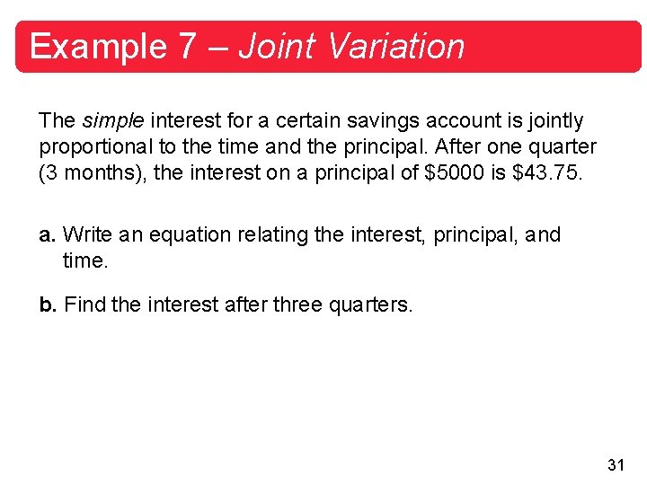
Example 7 – Joint Variation The simple interest for a certain savings account is jointly proportional to the time and the principal. After one quarter (3 months), the interest on a principal of $5000 is $43. 75. a. Write an equation relating the interest, principal, and time. b. Find the interest after three quarters. 31

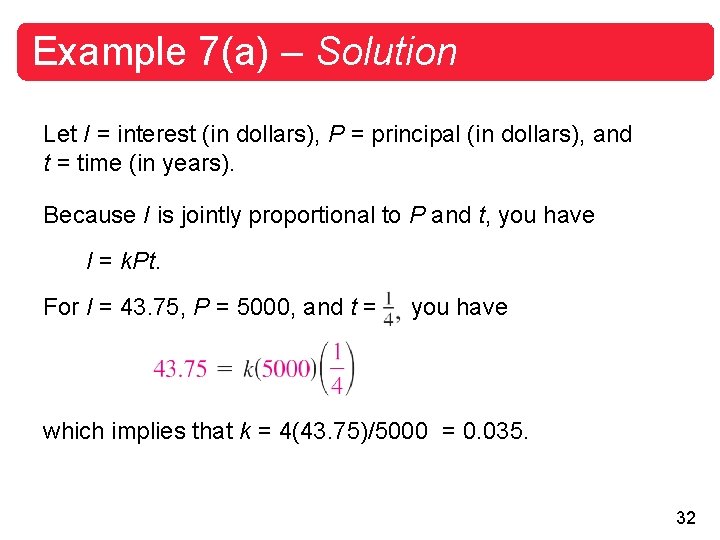
Example 7(a) – Solution Let I = interest (in dollars), P = principal (in dollars), and t = time (in years). Because I is jointly proportional to P and t, you have I = k. Pt. For I = 43. 75, P = 5000, and t = you have which implies that k = 4(43. 75)/5000 = 0. 035. 32

Example 7(a) – Solution cont’d So, the equation relating interest, principal, and time is I = 0. 035 P t which is the familiar equation for simple interest where the constant of proportionality, 0. 035, represents an annual interest rate of 3. 5%. 33

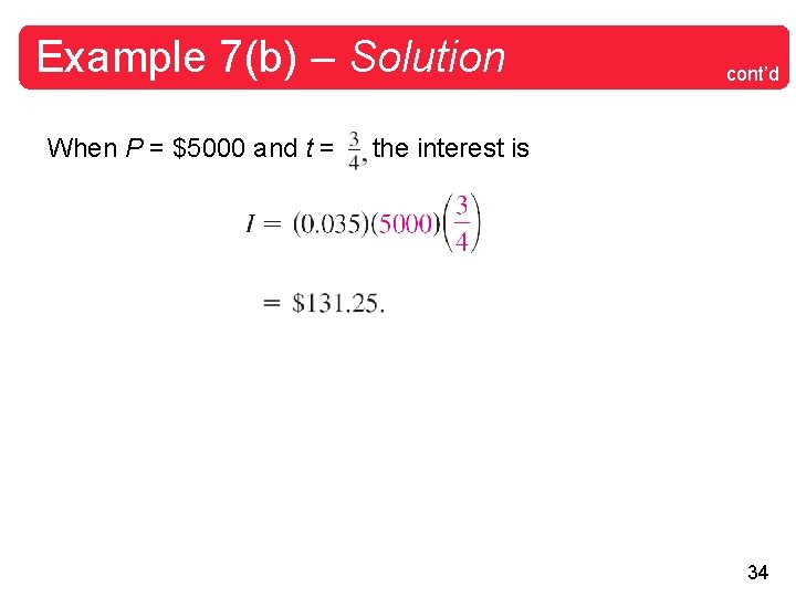
Example 7(b) – Solution When P = $5000 and t = cont’d the interest is 34