Functions and Their Graphs Copyright Cengage Learning All

Functions and Their Graphs Copyright © Cengage Learning. All rights reserved. 1

1. 10 MATHEMATICAL MODELING AND VARIATION Copyright © Cengage Learning. All rights reserved.

What You Should Learn • Use mathematical models to approximate sets of data points. • Use the regression feature of a graphing utility to find the equation of a least squares regression line. • Write mathematical models for direct variation. 3

What You Should Learn • Write mathematical models for direct variation as an nth power. • Write mathematical models for inverse variation. • Write mathematical models for joint variation. 4

Introduction 5

Introduction We have already studied some techniques for fitting models to data. For instance, we have learned how to find the equation of a line that passes through two points. In this section, you will study other techniques for fitting models to data: least squares regression and direct and inverse variation. The resulting models are either polynomial functions or rational functions. 6

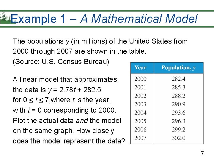
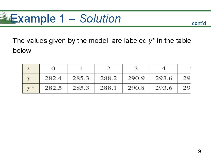
Example 1 – A Mathematical Model The populations y (in millions) of the United States from 2000 through 2007 are shown in the table. (Source: U. S. Census Bureau) A linear model that approximates the data is y = 2. 78 t + 282. 5 for 0 t 7, where t is the year, with t = 0 corresponding to 2000. Plot the actual data and the model on the same graph. How closely does the model represent the data? 7

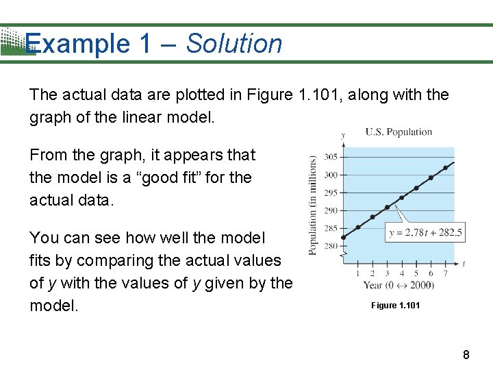
Example 1 – Solution The actual data are plotted in Figure 1. 101, along with the graph of the linear model. From the graph, it appears that the model is a “good fit” for the actual data. You can see how well the model fits by comparing the actual values of y with the values of y given by the model. Figure 1. 101 8

Example 1 – Solution cont’d The values given by the model are labeled y* in the table below. 9

Introduction Note in Example 1 that you could have chosen any two points to find a line that fits the data. However, the given linear model was found using the regression feature of a graphing utility and is the line that best fits the data. 10

Least Squares Regression and Graphing Utilities 11

Least Squares Regression and Graphing Utilities You have worked with many different types of mathematical models that approximate real-life data. In some instances the model was given (as in Example 1), whereas in other instances you were asked to find the model using simple algebraic techniques or a graphing utility. To find a model that approximates the data most accurately, statisticians use a measure called the sum of square differences, which is the sum of the squares of the differences between actual data values and model values. 12

Least Squares Regression and Graphing Utilities The “best-fitting” linear model, called the least squares regression line, is the one with the least sum of square differences. Recall that you can approximate this line visually by plotting the data points and drawing the line that appears to fit best —or you can enter the data points into a calculator or computer and use the linear regression feature of the calculator or computer. 13

Least Squares Regression and Graphing Utilities When you use the regression feature of a graphing calculator or computer program, you will notice that the program may also output an “r -value. ” This r -value is the correlation coefficient of the data and gives a measure of how well the model fits the data. The closer the value of | r | is to 1, the better the fit. 14

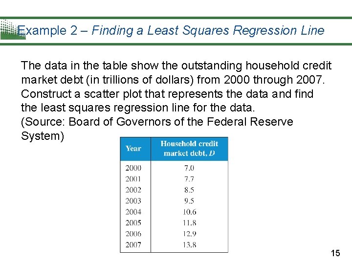
Example 2 – Finding a Least Squares Regression Line The data in the table show the outstanding household credit market debt (in trillions of dollars) from 2000 through 2007. Construct a scatter plot that represents the data and find the least squares regression line for the data. (Source: Board of Governors of the Federal Reserve System) 15

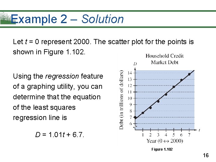
Example 2 – Solution Let t = 0 represent 2000. The scatter plot for the points is shown in Figure 1. 102. Using the regression feature of a graphing utility, you can determine that the equation of the least squares regression line is D = 1. 01 t + 6. 7. Figure 1. 102 16

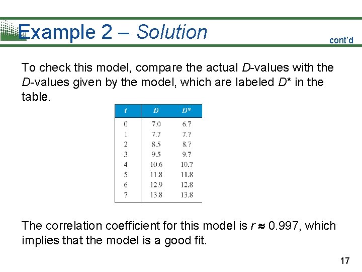
Example 2 – Solution cont’d To check this model, compare the actual D-values with the D-values given by the model, which are labeled D* in the table. The correlation coefficient for this model is r 0. 997, which implies that the model is a good fit. 17

Direct Variation 18

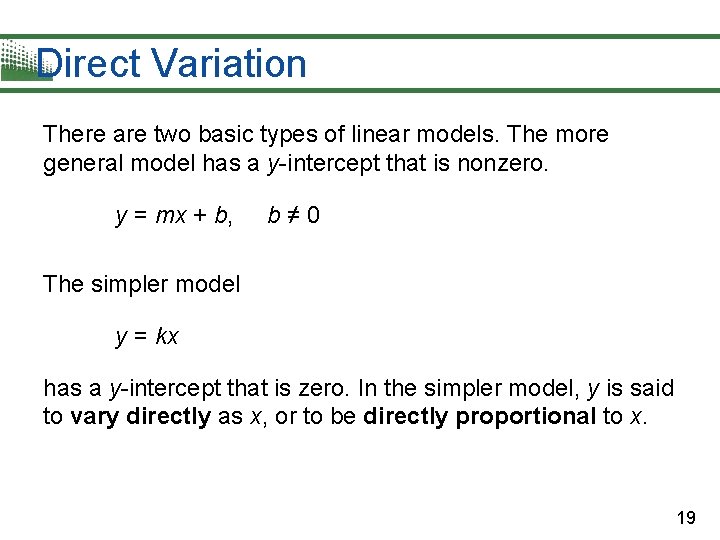
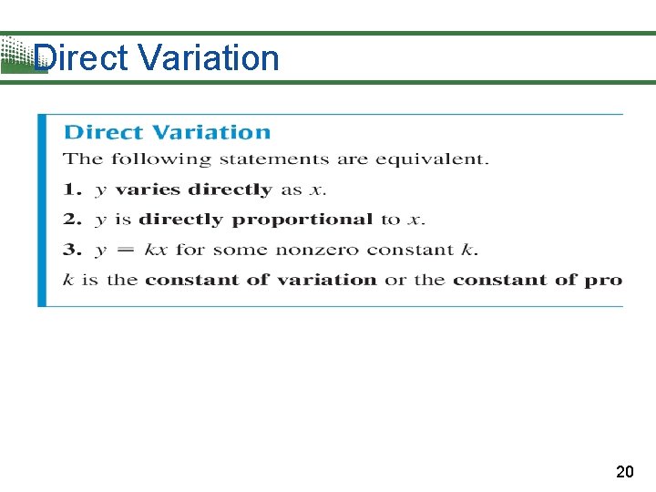
Direct Variation There are two basic types of linear models. The more general model has a y-intercept that is nonzero. y = mx + b, b≠ 0 The simpler model y = kx has a y-intercept that is zero. In the simpler model, y is said to vary directly as x, or to be directly proportional to x. 19

Direct Variation 20

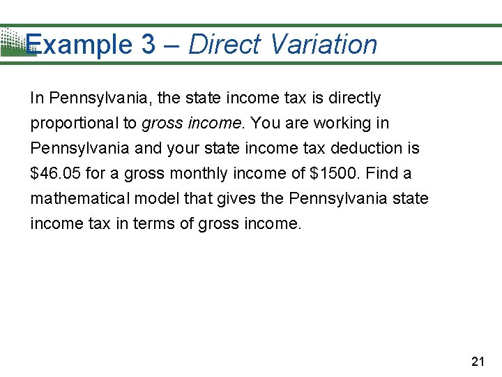
Example 3 – Direct Variation In Pennsylvania, the state income tax is directly proportional to gross income. You are working in Pennsylvania and your state income tax deduction is $46. 05 for a gross monthly income of $1500. Find a mathematical model that gives the Pennsylvania state income tax in terms of gross income. 21

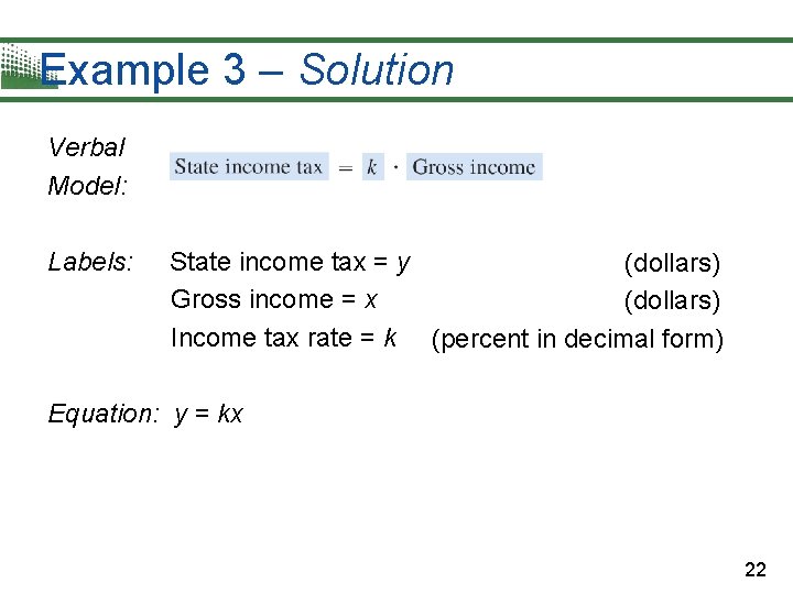
Example 3 – Solution Verbal Model: Labels: State income tax = y (dollars) Gross income = x (dollars) Income tax rate = k (percent in decimal form) Equation: y = kx 22

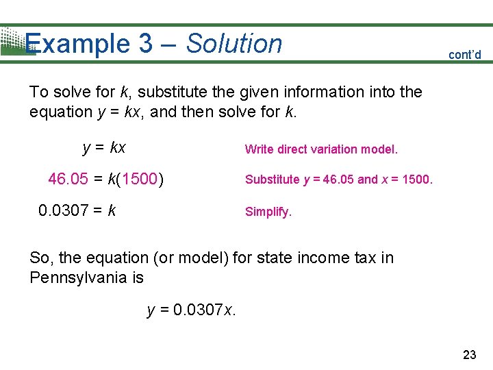
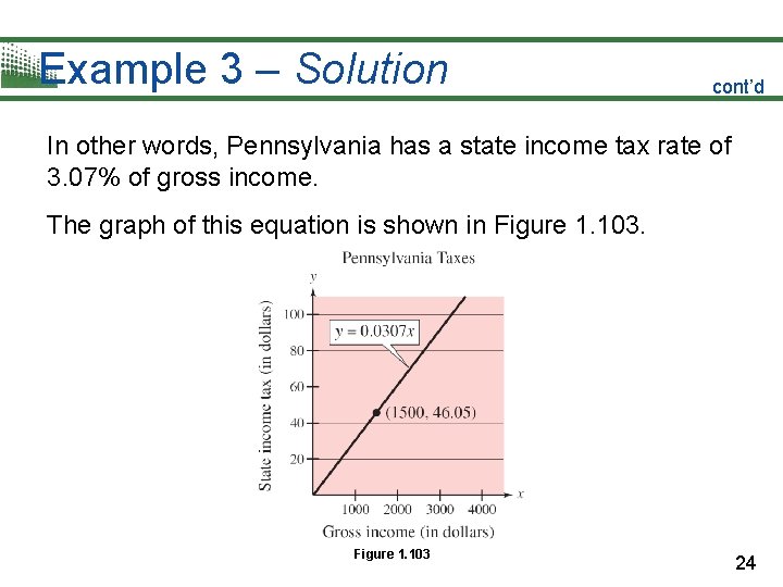
Example 3 – Solution cont’d To solve for k, substitute the given information into the equation y = kx, and then solve for k. y = kx Write direct variation model. 46. 05 = k(1500) 0. 0307 = k Substitute y = 46. 05 and x = 1500. Simplify. So, the equation (or model) for state income tax in Pennsylvania is y = 0. 0307 x. 23

Example 3 – Solution cont’d In other words, Pennsylvania has a state income tax rate of 3. 07% of gross income. The graph of this equation is shown in Figure 1. 103 24

Direct Variation as an nth Power 25

Direct Variation as an nth Power Another type of direct variation relates one variable to a power of another variable. For example, in the formula for the area of a circle A = r 2 the area A is directly proportional to the square of the radius r. Note that for this formula, is the constant of proportionality. 26

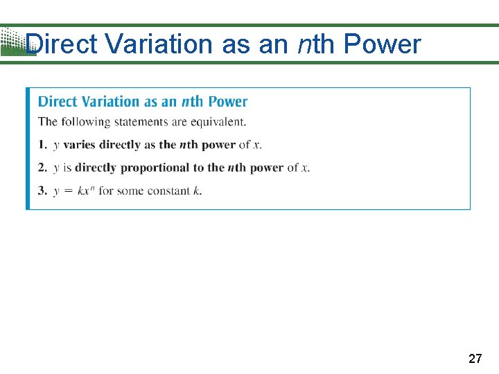
Direct Variation as an nth Power 27

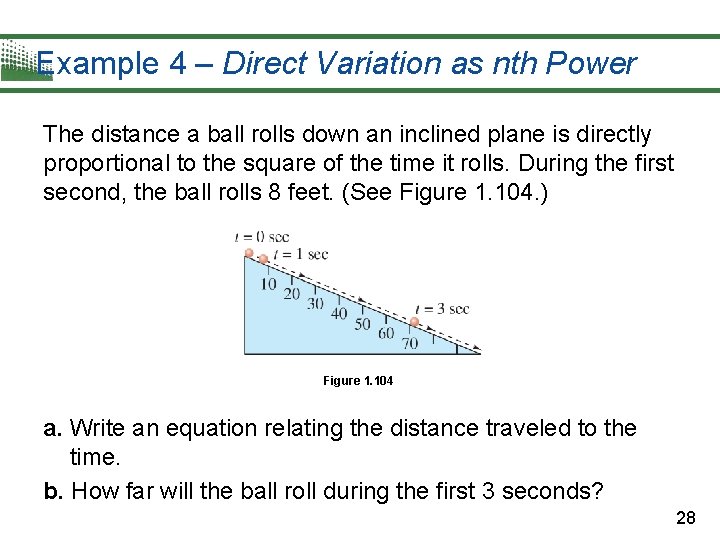
Example 4 – Direct Variation as nth Power The distance a ball rolls down an inclined plane is directly proportional to the square of the time it rolls. During the first second, the ball rolls 8 feet. (See Figure 1. 104. ) Figure 1. 104 a. Write an equation relating the distance traveled to the time. b. How far will the ball roll during the first 3 seconds? 28

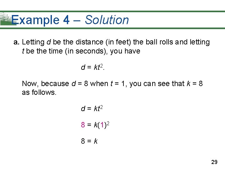
Example 4 – Solution a. Letting d be the distance (in feet) the ball rolls and letting t be the time (in seconds), you have d = kt 2. Now, because d = 8 when t = 1, you can see that k = 8 as follows. d = kt 2 8 = k(1)2 8=k 29

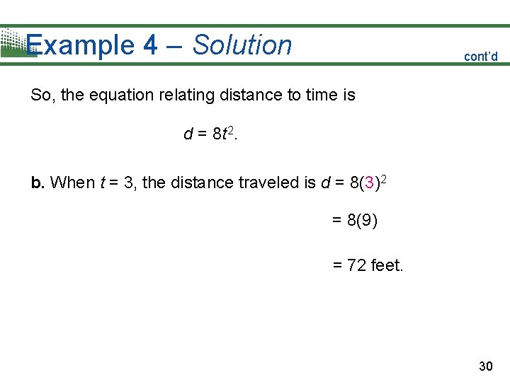
Example 4 – Solution cont’d So, the equation relating distance to time is d = 8 t 2. b. When t = 3, the distance traveled is d = 8(3)2 = 8(9) = 72 feet. 30

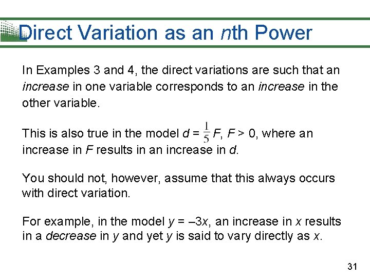
Direct Variation as an nth Power In Examples 3 and 4, the direct variations are such that an increase in one variable corresponds to an increase in the other variable. This is also true in the model d = F, F > 0, where an increase in F results in an increase in d. You should not, however, assume that this always occurs with direct variation. For example, in the model y = – 3 x, an increase in x results in a decrease in y and yet y is said to vary directly as x. 31

Inverse Variation 32

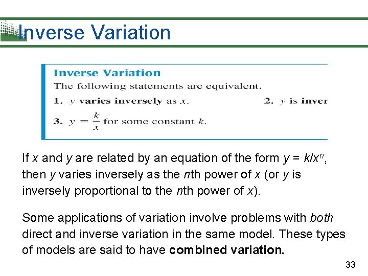
Inverse Variation If x and y are related by an equation of the form y = k/x n, then y varies inversely as the nth power of x (or y is inversely proportional to the nth power of x). [ Some applications of variation involve problems with both direct and inverse variation in the same model. These types of models are said to have combined variation. 33

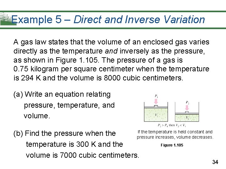
Example 5 – Direct and Inverse Variation A gas law states that the volume of an enclosed gas varies directly as the temperature and inversely as the pressure, as shown in Figure 1. 105. The pressure of a gas is 0. 75 kilogram per square centimeter when the temperature is 294 K and the volume is 8000 cubic centimeters. (a) Write an equation relating pressure, temperature, and volume. If the temperature is held constant and (b) Find the pressure when the pressure increases, volume decreases. Figure 1. 105 temperature is 300 K and the volume is 7000 cubic centimeters. 34

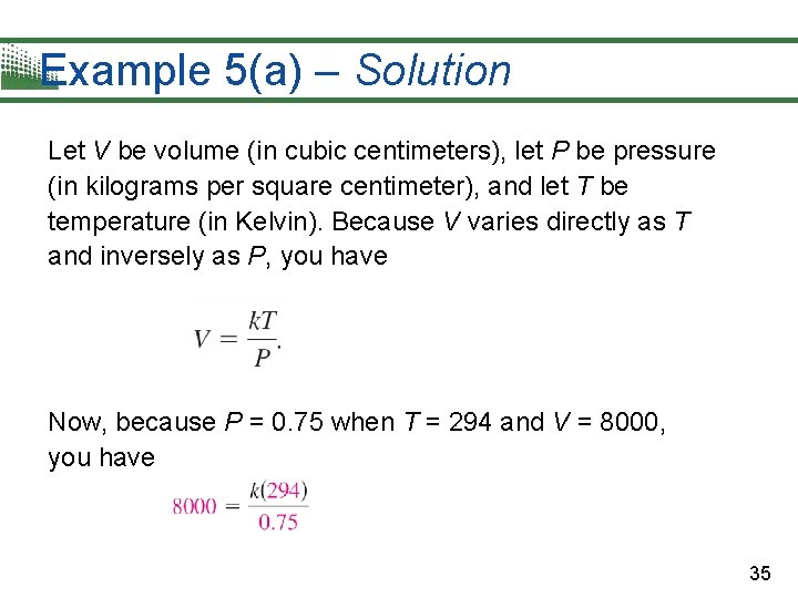
Example 5(a) – Solution Let V be volume (in cubic centimeters), let P be pressure (in kilograms per square centimeter), and let T be temperature (in Kelvin). Because V varies directly as T and inversely as P, you have Now, because P = 0. 75 when T = 294 and V = 8000, you have 35

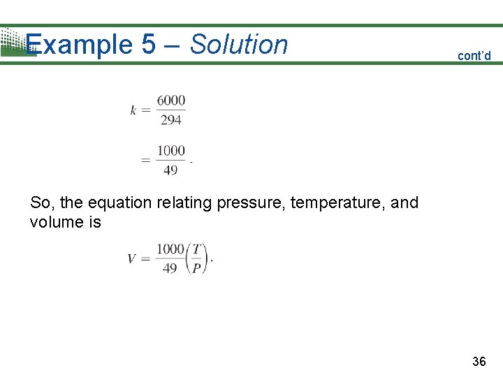
Example 5 – Solution cont’d So, the equation relating pressure, temperature, and volume is 36

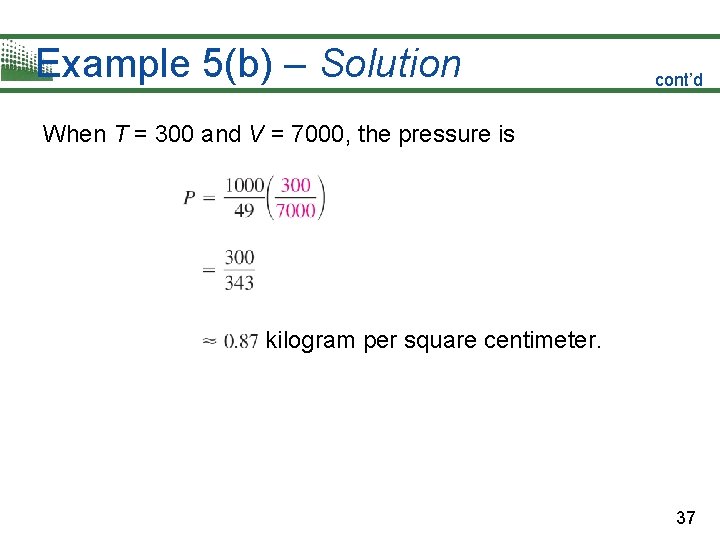
Example 5(b) – Solution cont’d When T = 300 and V = 7000, the pressure is kilogram per square centimeter. 37

Joint Variation 38

Joint Variation In Example 5, note that when a direct variation and an inverse variation occur in the same statement, they are coupled with the word “and. ” To describe two different direct variations in the same statement, the word jointly is used. 39

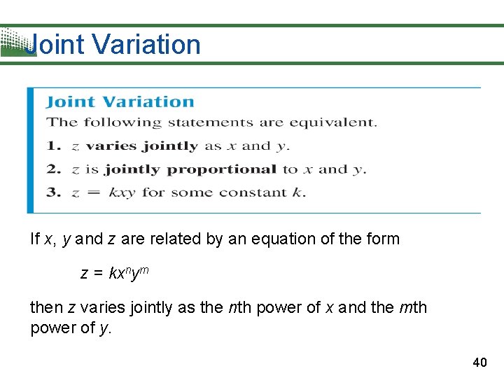
Joint Variation If x, y and z are related by an equation of the form z = kxnym then z varies jointly as the nth power of x and the mth power of y. 40

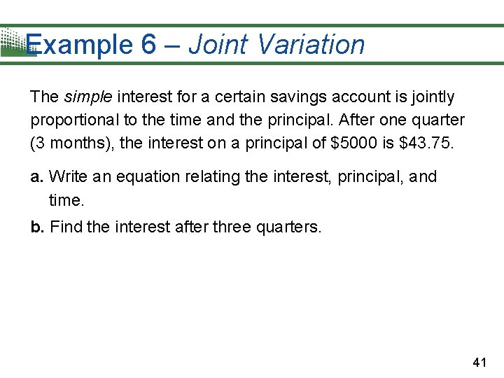
Example 6 – Joint Variation The simple interest for a certain savings account is jointly proportional to the time and the principal. After one quarter (3 months), the interest on a principal of $5000 is $43. 75. a. Write an equation relating the interest, principal, and time. b. Find the interest after three quarters. 41

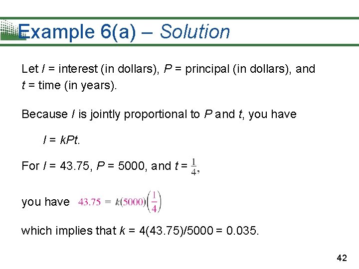
Example 6(a) – Solution Let I = interest (in dollars), P = principal (in dollars), and t = time (in years). Because I is jointly proportional to P and t, you have I = k. Pt. For I = 43. 75, P = 5000, and t = you have which implies that k = 4(43. 75)/5000 = 0. 035. 42

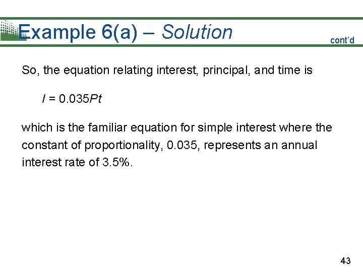
Example 6(a) – Solution cont’d So, the equation relating interest, principal, and time is I = 0. 035 P t which is the familiar equation for simple interest where the constant of proportionality, 0. 035, represents an annual interest rate of 3. 5%. 43

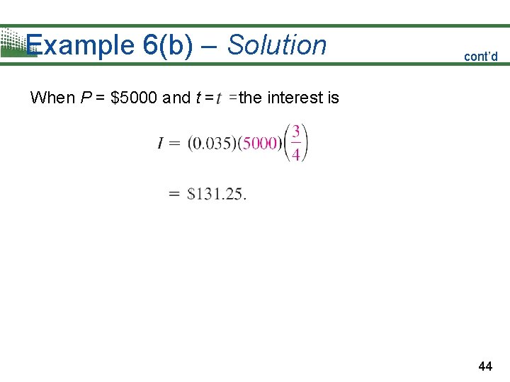
Example 6(b) – Solution When P = $5000 and t = cont’d the interest is 44