Polynomial Functions and their Graphs Section 3 1

Polynomial Functions and their Graphs Section 3. 1

General Shape of Polynomial Graphs l l The graph of polynomials are smooth, unbroken lines or curves, with no sharp corners or cusps (see p. 251). Every Polynomial function is defined and continuous for all real numbers.

Review l General polynomial formula l l a 0, a 1, … , an are constant coefficients n is the degree of the polynomial Standard form is for descending powers of x anxn is said to be the “leading term” term

Family of Polynomials l Constant polynomial functions l l Linear polynomial functions l l f(x) = a f(x) = mx + b Quadratic polynomial functions l f(x) = ax 2 + bx + c

Family of Polynomials l Cubic polynomial functions l l l f(x) = a x 3 + b x 2 + c x + d 3 rd degree polynomial Quartic polynomial functions l l f(x) = a x 4 + b x 3 + c x 2+ d x + e 4 th degree polynomial

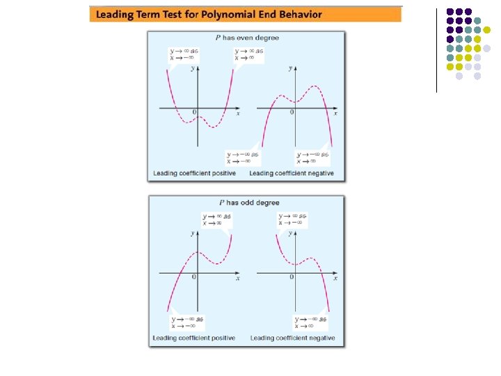
Polynomial “End Behavior” Behavior l Consider what happens when x gets very large in positive and negative direction l l Called “end behavior” Also “long-run” behavior Basically, the leading term anxn dominates the shape of graph There are 4 possible scenarios:

End Behavior Discuss end behavior for the following graphs: l l l

Compare Graph Behavior Consider the following graphs: l f(x) = x 4 - 4 x 3 + 16 x - 16 l g(x) = x 4 - 4 x 3 - 4 x 2 +16 x l h(x) = x 4 + x 3 - 8 x 2 - 12 x l Graph these on the window -8 < x < 8 and 0 < y < 4000 l Decide how these functions are alike or different, based on the view of this graph

Compare Graph Behavior l From this view, they appear very similar

Compare “Short Run” Behavior l Now Change the window to be -5 < x < 5 and -35 < y < 15 l How do the functions appear to be different from this view?

Compare Short Run Behavior Differences? l Real zeros l Local extrema l Complex zeros l Note: The standard form of the polynomials does not give any clues as to this short run behavior of the polynomials:

Using Zeros to Graph Polynomials l Consider the following polynomial: l l What will the zeros be for this polynomial? l l p(x) = (x - 2)(2 x + 3)(x + 5) x = 2 x = -3/2 x = -5 How do you know? l Zero-Factor Property: If a*b = 0 then, we know that either a = 0 or b = 0 (or both)

Guidelines to Graphing l l Zeros Test Points (like table of signs) End Behavior Graph (a smooth curve through all known points)

Intermediate Value Theorem l If P is a polynomial function and P(a) and P(b) have opposite signs, then there is at least one value c between a and b for which P(c) = 0.

Theorem l Local Extrema of Polynomial Functions: l A polynomial function of degree n has at most n - 1 local extrema.

Local Extrema (turning points) l Local Extrema – a point (x, y) on the graph where the graph changes from increasing to decreasing or vice-versa. • •