1 Different architectures Two degreesoffreedom control Feedforward control

1. Different architectures • Two degrees-of-freedom control • Feedforward control • Addressing multiple inputs • Addressing complexity with multiple loops 2. More design with MATLAB ME 431, Lecture 24: More Advanced Architectures

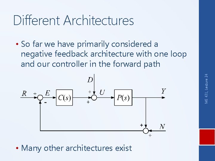
Different Architectures ME 431, Lecture 24 • So far we have primarily considered a negative feedback architecture with one loop and our controller in the forward path • Many other architectures exist

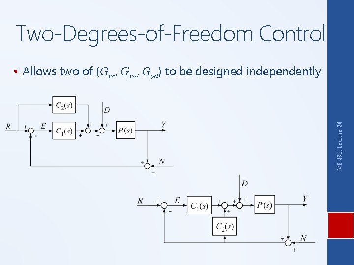
Two-Degrees-of-Freedom Control ME 431, Lecture 24 • Allows two of (Gyr, Gyn, Gyd) to be designed independently

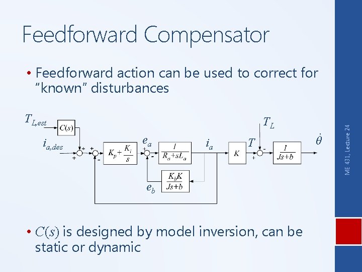
Feedforward Compensator TL, est ia, des TL ea ia T eb • C(s) is designed by model inversion, can be static or dynamic . θ ME 431, Lecture 24 • Feedforward action can be used to correct for “known” disturbances

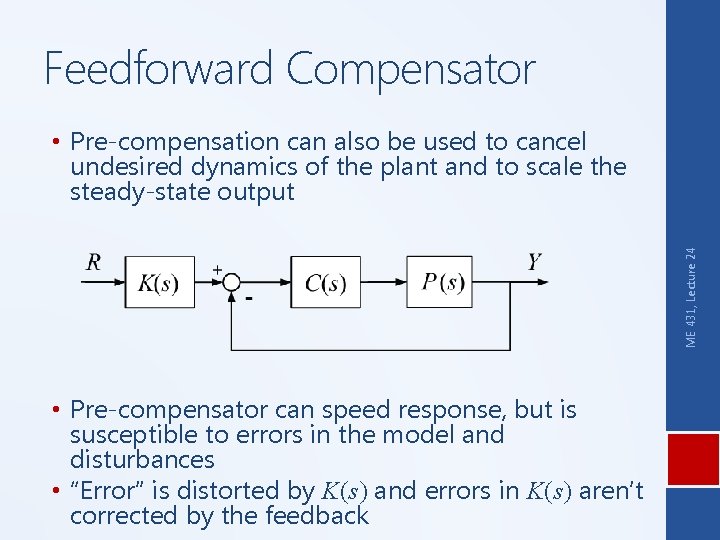
Feedforward Compensator ME 431, Lecture 24 • Pre-compensation can also be used to cancel undesired dynamics of the plant and to scale the steady-state output • Pre-compensator can speed response, but is susceptible to errors in the model and disturbances • “Error” is distorted by K(s) and errors in K(s) aren’t corrected by the feedback

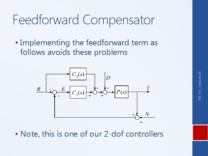
Feedforward Compensator ME 431, Lecture 24 • Implementing the feedforward term as follows avoids these problems • Note, this is one of our 2 -dof controllers

Multiple Inputs • When we had multiple inputs, we could examine the response to each input separately if the system was linear • If inputs are coupled in a nonlinear manner, we can use heuristics to decouple them ME 431, Lecture 24 • We have primarily designed control for single input single output (SISO) systems

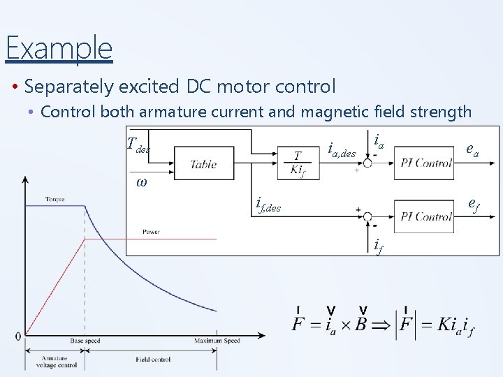
Example • Separately excited DC motor control • Control both armature current and magnetic field strength Tdes ia, des ia ea ω if, des ef if

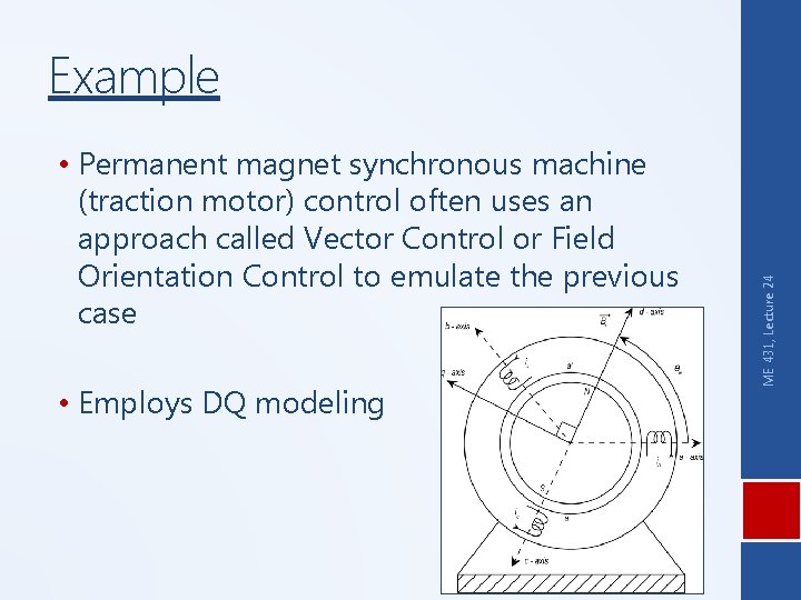
• Permanent magnet synchronous machine (traction motor) control often uses an approach called Vector Control or Field Orientation Control to emulate the previous case • Employs DQ modeling ME 431, Lecture 24 Example

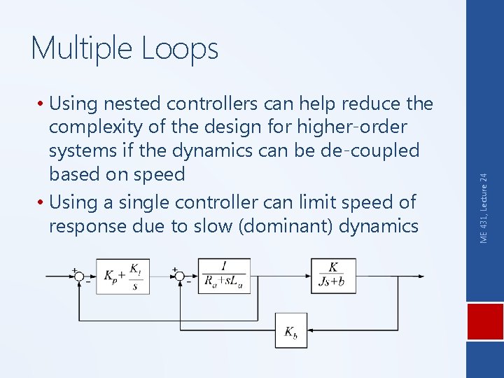
• Using nested controllers can help reduce the complexity of the design for higher-order systems if the dynamics can be de-coupled based on speed • Using a single controller can limit speed of response due to slow (dominant) dynamics ME 431, Lecture 24 Multiple Loops

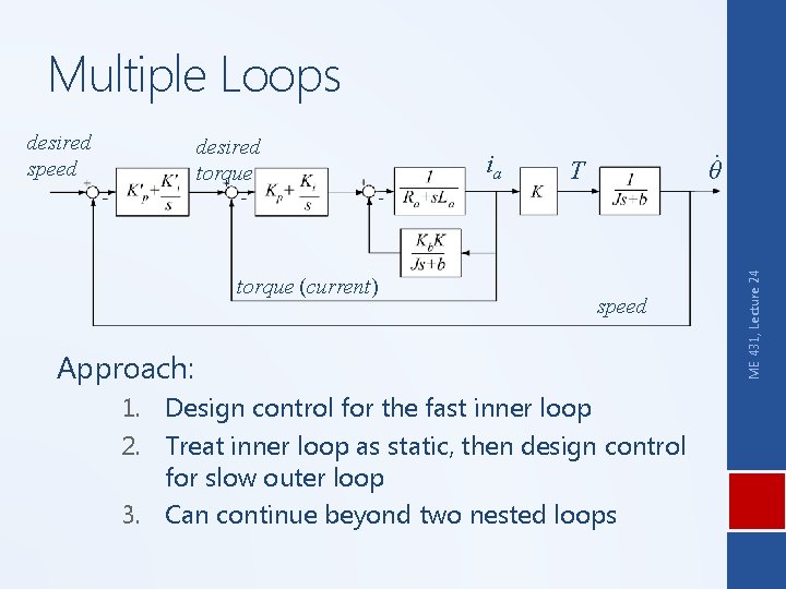
Multiple Loops desired torque (current) ia . θ T speed Approach: 1. Design control for the fast inner loop 2. Treat inner loop as static, then design control for slow outer loop 3. Can continue beyond two nested loops ME 431, Lecture 24 desired speed

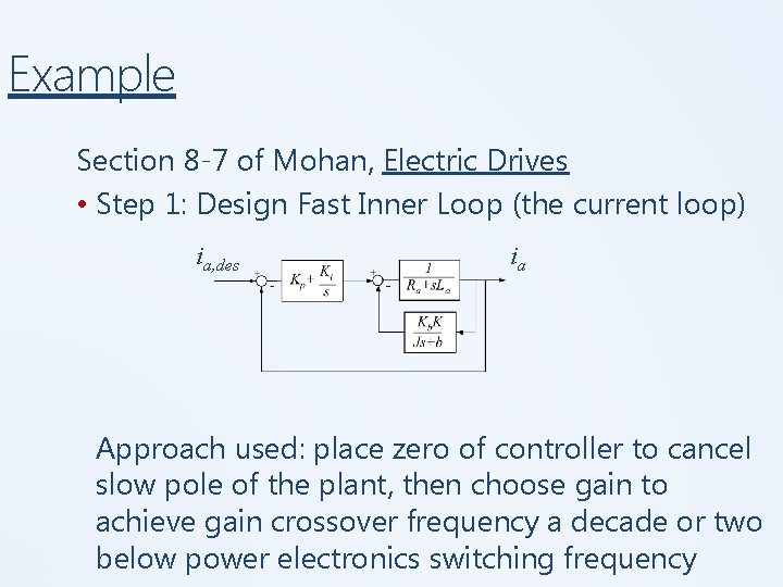
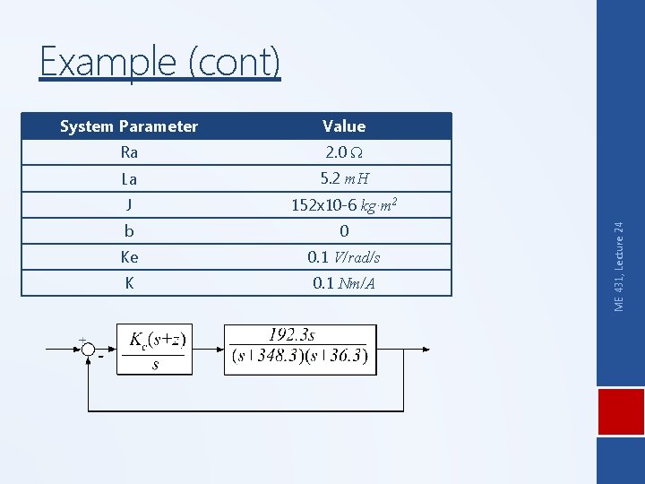
Example Section 8 -7 of Mohan, Electric Drives • Step 1: Design Fast Inner Loop (the current loop) ia, des ia Approach used: place zero of controller to cancel slow pole of the plant, then choose gain to achieve gain crossover frequency a decade or two below power electronics switching frequency

System Parameter Value Ra 2. 0 Ω La 5. 2 m. H J 152 x 10 -6 kg·m 2 b 0 Ke 0. 1 V/rad/s K 0. 1 Nm/A ME 431, Lecture 24 Example (cont)

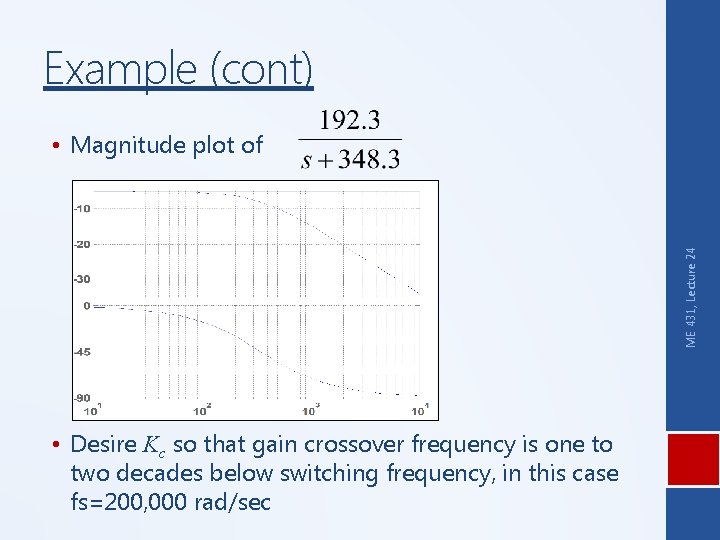
Example (cont) ME 431, Lecture 24 • Magnitude plot of • Desire Kc so that gain crossover frequency is one to two decades below switching frequency, in this case fs=200, 000 rad/sec

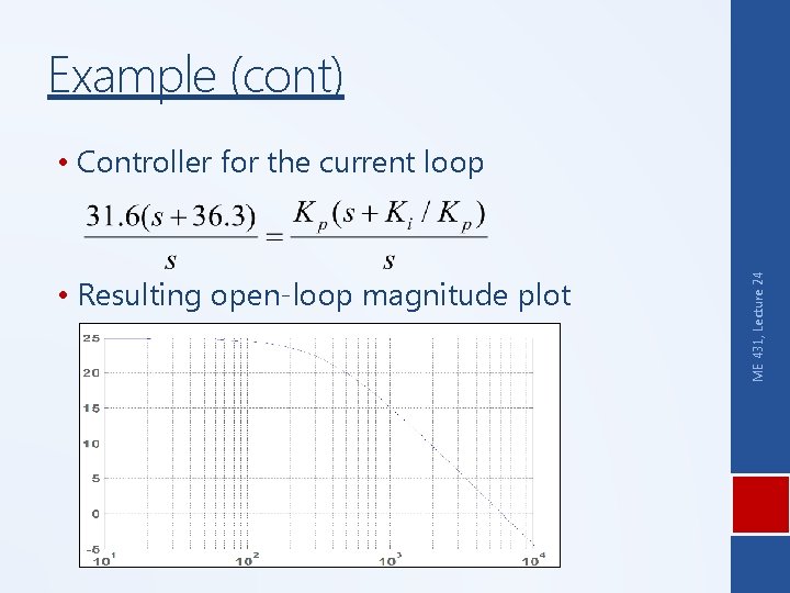
Example (cont) • Resulting open-loop magnitude plot ME 431, Lecture 24 • Controller for the current loop

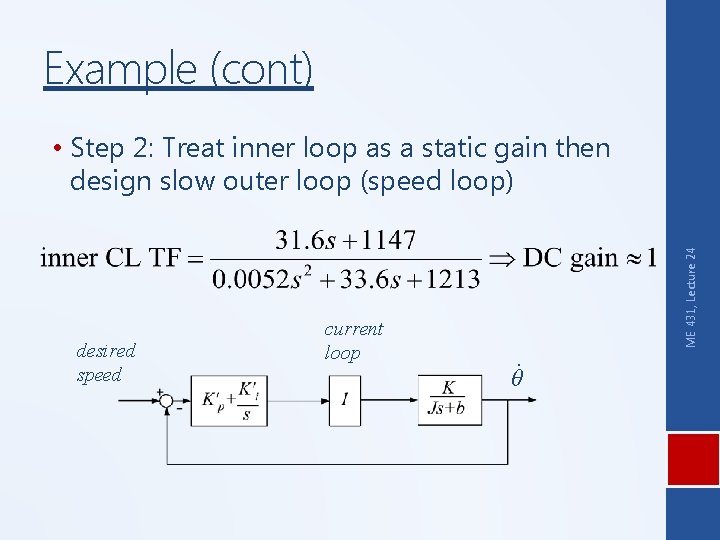
Example (cont) desired speed current loop . θ ME 431, Lecture 24 • Step 2: Treat inner loop as a static gain then design slow outer loop (speed loop)

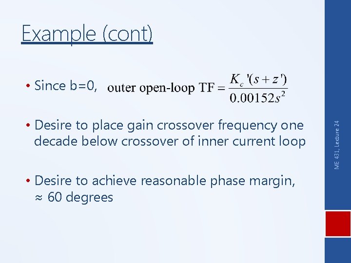
Example (cont) • Desire to place gain crossover frequency one decade below crossover of inner current loop • Desire to achieve reasonable phase margin, ≈ 60 degrees ME 431, Lecture 24 • Since b=0,

Example (cont) ME 431, Lecture 24 • Will use SISO Design tool in MATLAB