1 CE 530 Molecular Simulation Lecture 13 Molecular

1 CE 530 Molecular Simulation Lecture 13 Molecular Dynamics in Other Ensembles David A. Kofke Department of Chemical Engineering SUNY Buffalo kofke@eng. buffalo. edu

2 Review ¡ Molecular dynamics is a numerical integration of the classical equations of motion ¡ Total energy is strictly conserved, so MD samples the NVE ensemble ¡ Dynamical behaviors can be measured by taking appropriate time averages over the simulation • Spontaneous fluctuations provide non-equilibrium condition for measurement of transport in equilibrium MD • Non-equilibrium MD can be used to get less noisy results, but requires mechanism to remove energy via heat transfer ¡ Two equivalent formalisms for EMD measurements • Einstein equation • Green-Kubo relation time correlation functions

3 Molecular Dynamics in Other Ensembles ¡ Standard MD samples the NVE ensemble ¡ There is need enable MD to operate at constant T and/or P • with standard MD it is very hard to set initial positions and velocities to give a desired T or P with any accuracy NPT MD permits control over state conditions of most interest • NEMD and other advanced methods require temperature control ¡ Two general approaches • stochastic coupling to a reservoir • feedback control ¡ Good methods ensure proper sampling of the appropriate ensemble

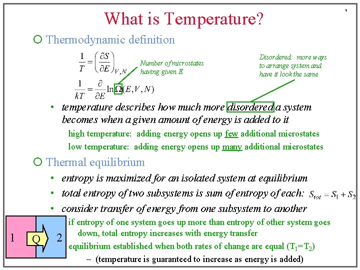
What is Temperature? ¡ Thermodynamic definition Number of microstates having given E Disordered: more ways to arrange system and have it look the same • temperature describes how much more disordered a system becomes when a given amount of energy is added to it high temperature: adding energy opens up few additional microstates low temperature: adding energy opens up many additional microstates ¡ Thermal equilibrium • entropy is maximized for an isolated system at equilibrium • total entropy of two subsystems is sum of entropy of each: • consider transfer of energy from one subsystem to another 1 Q 2 if entropy of one system goes up more than entropy of other system goes down, total entropy increases with energy transfer equilibrium established when both rates of change are equal (T 1=T 2) – (temperature is guaranteed to increase as energy is added) 4

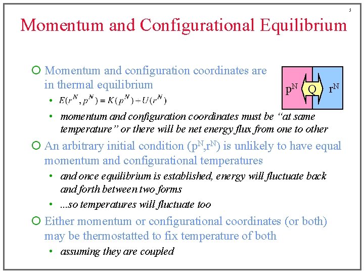
5 Momentum and Configurational Equilibrium ¡ Momentum and configuration coordinates are in thermal equilibrium p. N Q • • momentum and configuration coordinates must be “at same temperature” or there will be net energy flux from one to other r. N ¡ An arbitrary initial condition (p. N, r. N) is unlikely to have equal momentum and configurational temperatures • and once equilibrium is established, energy will fluctuate back and forth between two forms • . . . so temperatures will fluctuate too ¡ Either momentum or configurational coordinates (or both) may be thermostatted to fix temperature of both • assuming they are coupled

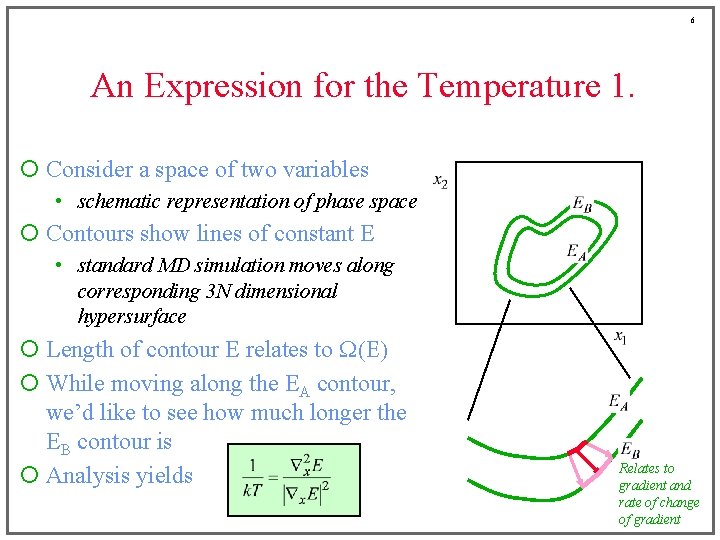
6 An Expression for the Temperature 1. ¡ Consider a space of two variables • schematic representation of phase space ¡ Contours show lines of constant E • standard MD simulation moves along corresponding 3 N dimensional hypersurface ¡ Length of contour E relates to W(E) ¡ While moving along the EA contour, we’d like to see how much longer the EB contour is ¡ Analysis yields Relates to gradient and rate of change of gradient

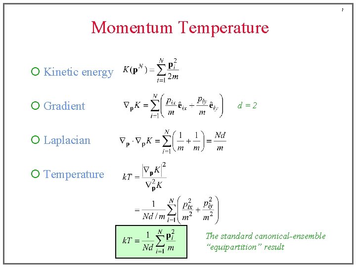
7 Momentum Temperature ¡ Kinetic energy ¡ Gradient d=2 ¡ Laplacian ¡ Temperature The standard canonical-ensemble “equipartition” result

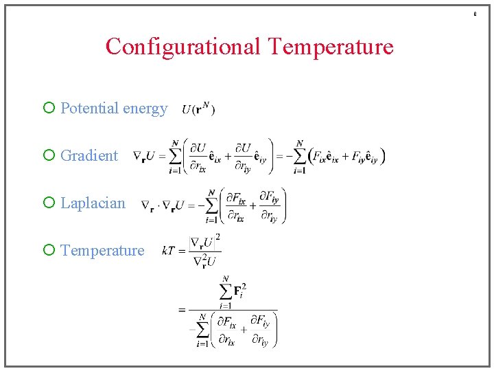
8 Configurational Temperature ¡ Potential energy ¡ Gradient ¡ Laplacian ¡ Temperature

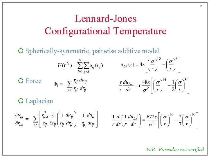
9 Lennard-Jones Configurational Temperature ¡ Spherically-symmetric, pairwise additive model ¡ Force ¡ Laplacian N. B. Formulas not verified

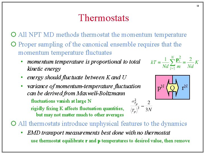
10 Thermostats ¡ All NPT MD methods thermostat the momentum temperature ¡ Proper sampling of the canonical ensemble requires that the momentum temperature fluctuates • momentum temperature is proportional to total kinetic energy • energy should fluctuate between K and U • variance of momentum-temperature fluctuation can be derived from Maxwell-Boltzmann p. N Q r. N fluctuations vanish at large N rigidly fixing K affects fluctuation quantities, but may not matter much to other averages ¡ All thermostats introduce unphysical features to the dynamics • EMD transport measurements best done with no thermostat use thermostat equilibrate r and p temperatures to desired value, then remove

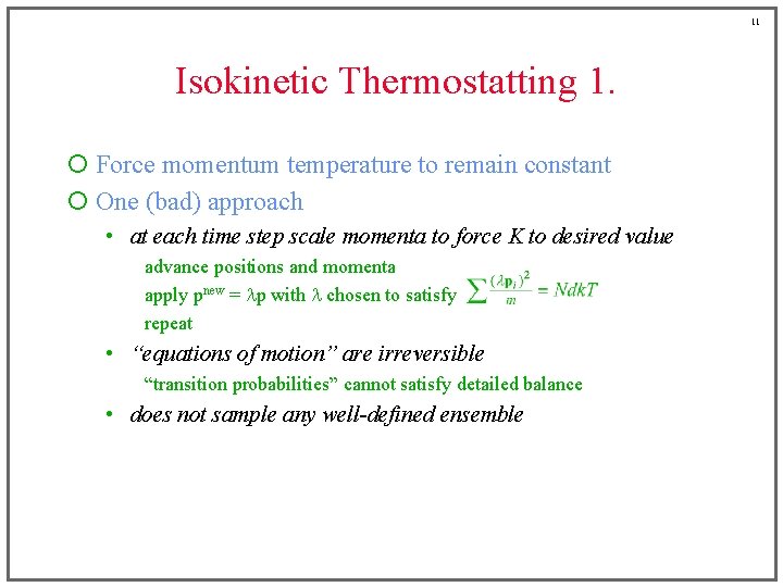
11 Isokinetic Thermostatting 1. ¡ Force momentum temperature to remain constant ¡ One (bad) approach • at each time step scale momenta to force K to desired value advance positions and momenta apply pnew = lp with l chosen to satisfy repeat • “equations of motion” are irreversible “transition probabilities” cannot satisfy detailed balance • does not sample any well-defined ensemble

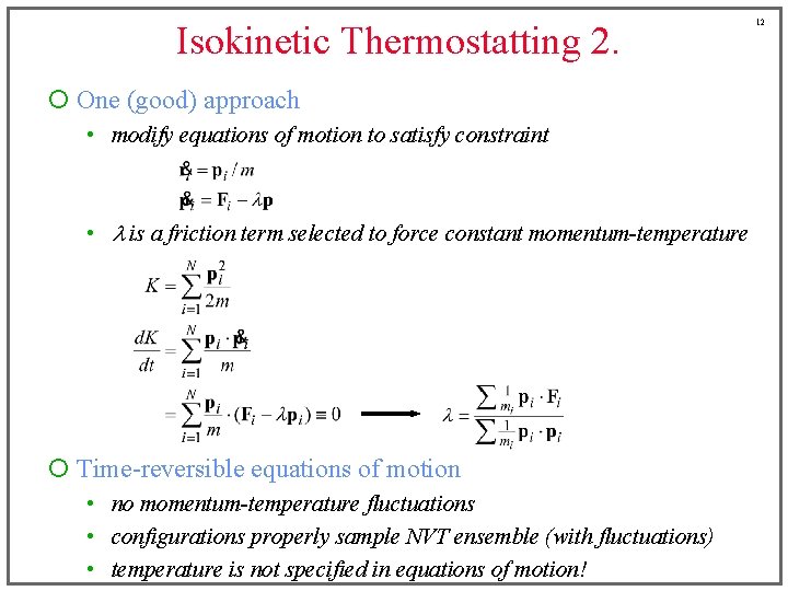
Isokinetic Thermostatting 2. ¡ One (good) approach • modify equations of motion to satisfy constraint • l is a friction term selected to force constant momentum-temperature ¡ Time-reversible equations of motion • no momentum-temperature fluctuations • configurations properly sample NVT ensemble (with fluctuations) • temperature is not specified in equations of motion! 12

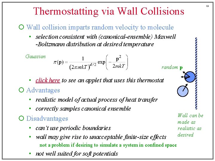
Thermostatting via Wall Collisions ¡ Wall collision imparts random velocity to molecule • selection consistent with (canonical-ensemble) Maxwell -Boltzmann distribution at desired temperature Gaussian random p • click here to see an applet that uses this thermostat ¡ Advantages • realistic model of actual process of heat transfer • correctly samples canonical ensemble ¡ Disadvantages • can’t use periodic boundaries • wall may give rise to unacceptable finite-size effects not a problem if desiring to simulate a system in confined space • not well suited for soft potentials Wall can be made as realistic as desired 13

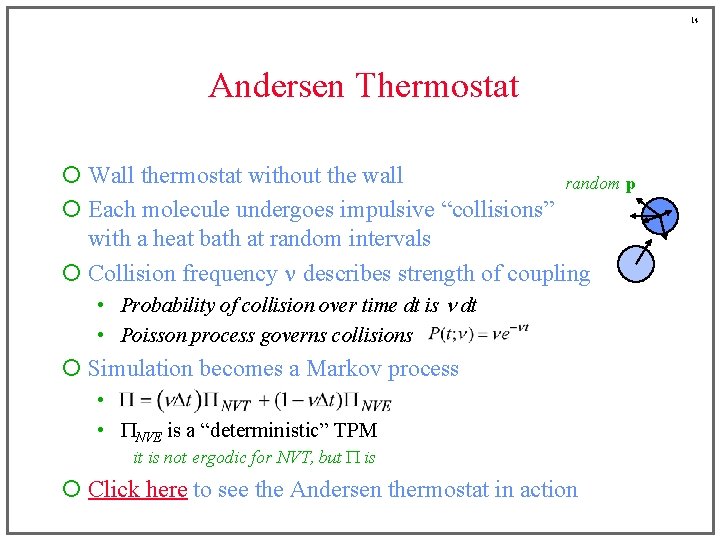
14 Andersen Thermostat ¡ Wall thermostat without the wall random p ¡ Each molecule undergoes impulsive “collisions” with a heat bath at random intervals ¡ Collision frequency n describes strength of coupling • Probability of collision over time dt is n dt • Poisson process governs collisions ¡ Simulation becomes a Markov process • • PNVE is a “deterministic” TPM it is not ergodic for NVT, but P is ¡ Click here to see the Andersen thermostat in action

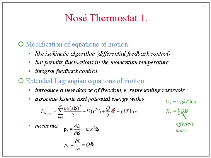
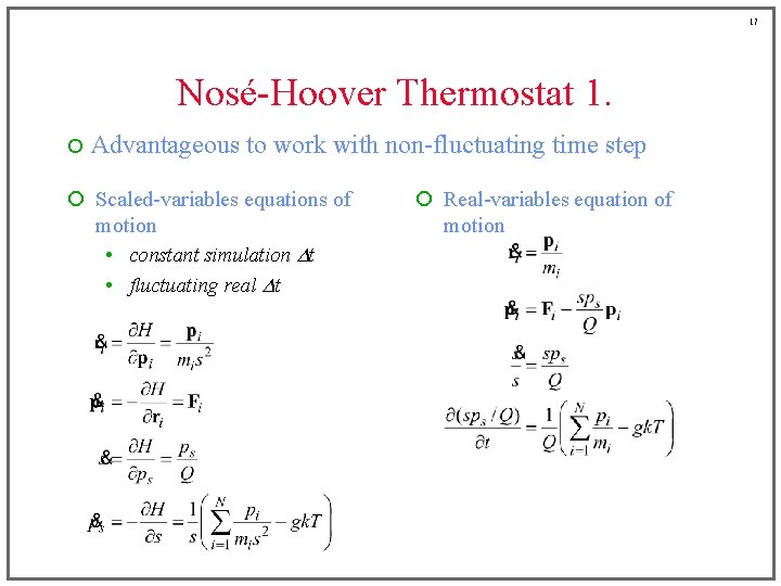
15 Nosé Thermostat 1. ¡ Modification of equations of motion • like isokinetic algorithm (differential feedback control) • but permits fluctuations in the momentum temperature • integral feedback control ¡ Extended Lagrangian equations of motion • introduce a new degree of freedom, s, representing reservoir • associate kinetic and potential energy with s • momenta effective mass

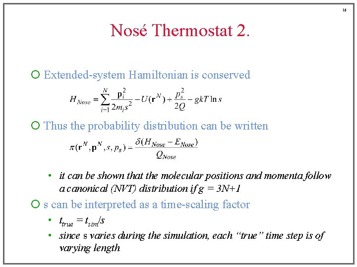
16 Nosé Thermostat 2. ¡ Extended-system Hamiltonian is conserved ¡ Thus the probability distribution can be written • it can be shown that the molecular positions and momenta follow a canonical (NVT) distribution if g = 3 N+1 ¡ s can be interpreted as a time-scaling factor • ttrue = tsim/s • since s varies during the simulation, each “true” time step is of varying length

17 Nosé-Hoover Thermostat 1. ¡ Advantageous to work with non-fluctuating time step ¡ Scaled-variables equations of motion • constant simulation Dt • fluctuating real Dt ¡ Real-variables equation of motion

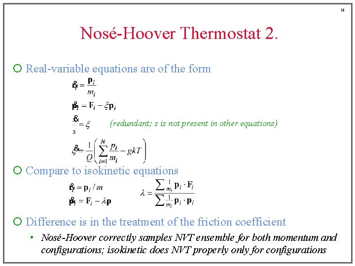
18 Nosé-Hoover Thermostat 2. ¡ Real-variable equations are of the form (redundant; s is not present in other equations) ¡ Compare to isokinetic equations ¡ Difference is in the treatment of the friction coefficient • Nosé-Hoover correctly samples NVT ensemble for both momentum and configurations; isokinetic does NVT properly only for configurations

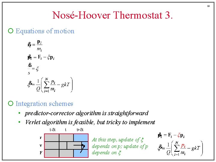
19 Nosé-Hoover Thermostat 3. ¡ Equations of motion ¡ Integration schemes • predictor-corrector algorithm is straightforward • Verlet algorithm is feasible, but tricky to implement t-dt r v F t t+dt At this step, update of x depends on p; update of p depends on x

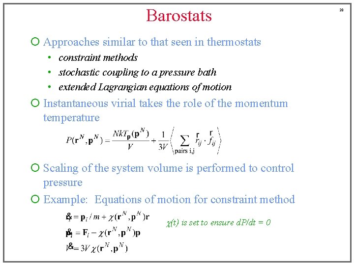
Barostats ¡ Approaches similar to that seen in thermostats • constraint methods • stochastic coupling to a pressure bath • extended Lagrangian equations of motion ¡ Instantaneous virial takes the role of the momentum temperature ¡ Scaling of the system volume is performed to control pressure ¡ Example: Equations of motion for constraint method c(t) is set to ensure d. P/dt = 0 20

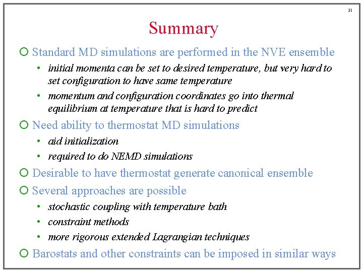
21 Summary ¡ Standard MD simulations are performed in the NVE ensemble • initial momenta can be set to desired temperature, but very hard to set configuration to have same temperature • momentum and configuration coordinates go into thermal equilibrium at temperature that is hard to predict ¡ Need ability to thermostat MD simulations • aid initialization • required to do NEMD simulations ¡ Desirable to have thermostat generate canonical ensemble ¡ Several approaches are possible • stochastic coupling with temperature bath • constraint methods • more rigorous extended Lagrangian techniques ¡ Barostats and other constraints can be imposed in similar ways