ECE 530 Analysis Techniques for LargeScale Electrical Systems

ECE 530 – Analysis Techniques for Large-Scale Electrical Systems Lecture 3: Power Flow Analysis Prof. Hao Zhu Dept. of Electrical and Computer Engineering University of Illinois at Urbana-Champaign haozhu@illinois. edu 1

Announcements • • Homework 1 will be posted today. Due Sep 11 (Thur), in class 2

Static Power System Analysis • • One of the most common power system analysis tools is the power flow, which tells how power flows through a power system in the quasi-steady state time frame The power flow can be used to model the full, threephase system, but usually (practically always) for transmission system analysis the system is assumed to be balanced. Hence a per phase equivalent model is used. 3

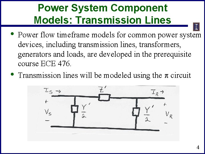
Power System Component Models: Transmission Lines • • Power flow timeframe models for common power system devices, including transmission lines, transformers, generators and loads, are developed in the prerequisite course ECE 476. Transmission lines will be modeled using the p circuit 4

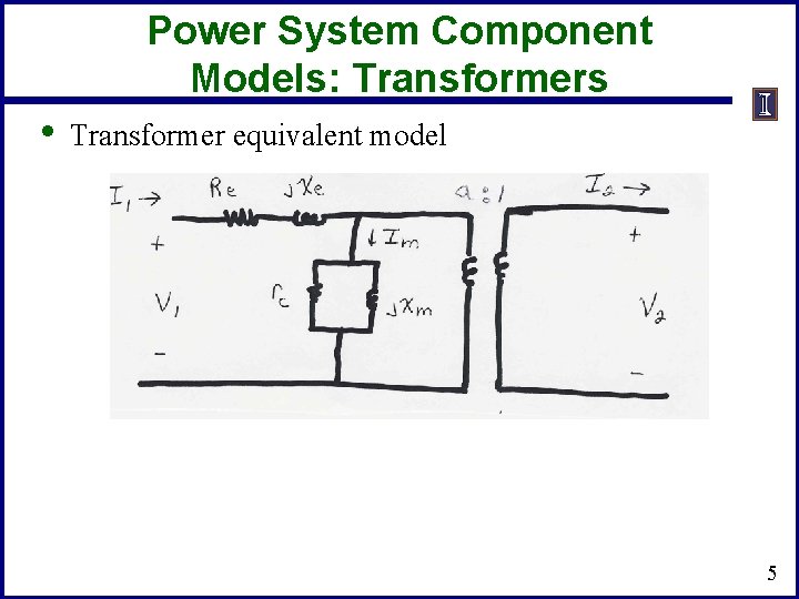
Power System Component Models: Transformers • Transformer equivalent model 5

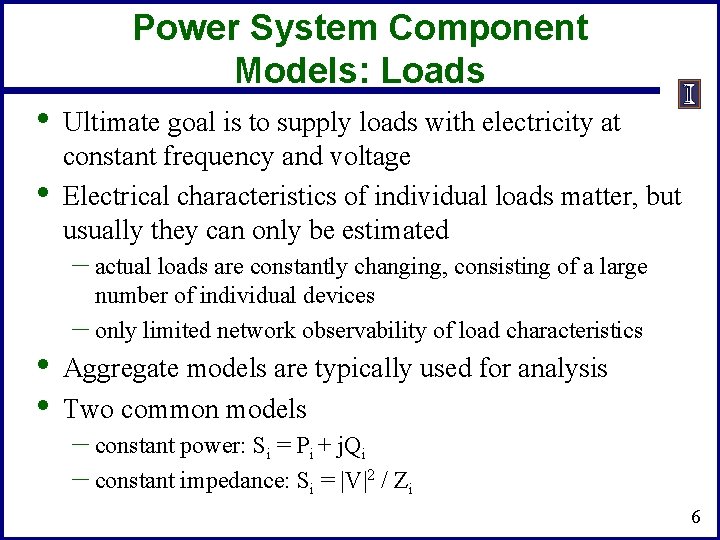
Power System Component Models: Loads • • Ultimate goal is to supply loads with electricity at constant frequency and voltage Electrical characteristics of individual loads matter, but usually they can only be estimated – actual loads are constantly changing, consisting of a large • • number of individual devices – only limited network observability of load characteristics Aggregate models are typically used for analysis Two common models – constant power: Si = Pi + j. Qi – constant impedance: Si = |V|2 / Zi 6

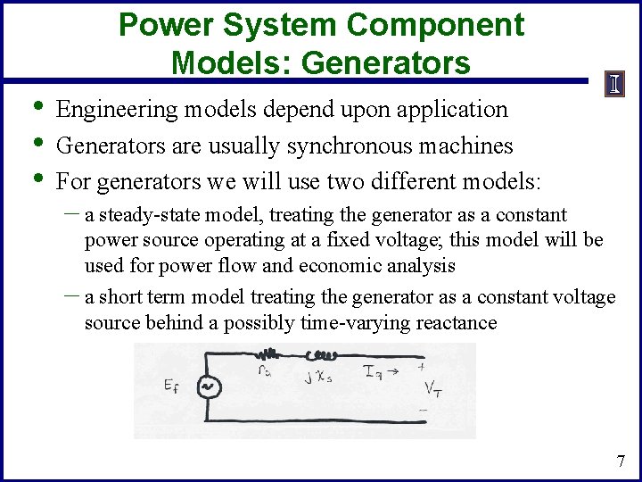
Power System Component Models: Generators • • • Engineering models depend upon application Generators are usually synchronous machines For generators we will use two different models: – a steady-state model, treating the generator as a constant power source operating at a fixed voltage; this model will be used for power flow and economic analysis – a short term model treating the generator as a constant voltage source behind a possibly time-varying reactance 7

Per Phase Calculations • A key problem in analyzing power systems is the large number of transformers. – It would be very difficult to continually have to refer • • impedances to the different sides of the transformers This problem is avoided by a normalization of all variables. This normalization is known as per unit analysis 8

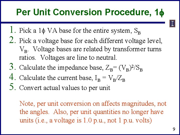
Per Unit Conversion Procedure, 1 f 1. Pick a 1 f VA base for the entire system, SB 2. Pick a voltage base for each different voltage level, 3. 4. 5. VB. Voltage bases are related by transformer turns ratios. Voltages are line to neutral. Calculate the impedance base, ZB= (VB)2/SB Calculate the current base, IB = VB/ZB Convert actual values to per unit Note, per unit conversion on affects magnitudes, not the angles. Also, per unit quantities no longer have units (i. e. , a voltage is 1. 0 p. u. , not 1 p. u. volts) 9

Per Unit Solution Procedure 1. 2. 3. Convert to per unit (p. u. ) (many problems are already in per unit) Solve Convert back to actual as necessary 10

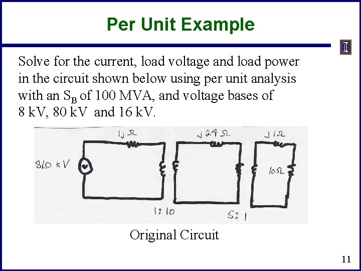
Per Unit Example Solve for the current, load voltage and load power in the circuit shown below using per unit analysis with an SB of 100 MVA, and voltage bases of 8 k. V, 80 k. V and 16 k. V. Original Circuit 11

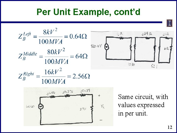
Per Unit Example, cont’d Same circuit, with values expressed in per unit. 12

Per Unit Example, cont’d 13

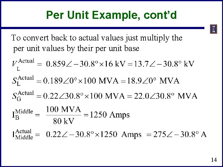
Per Unit Example, cont’d To convert back to actual values just multiply the per unit values by their per unit base 14

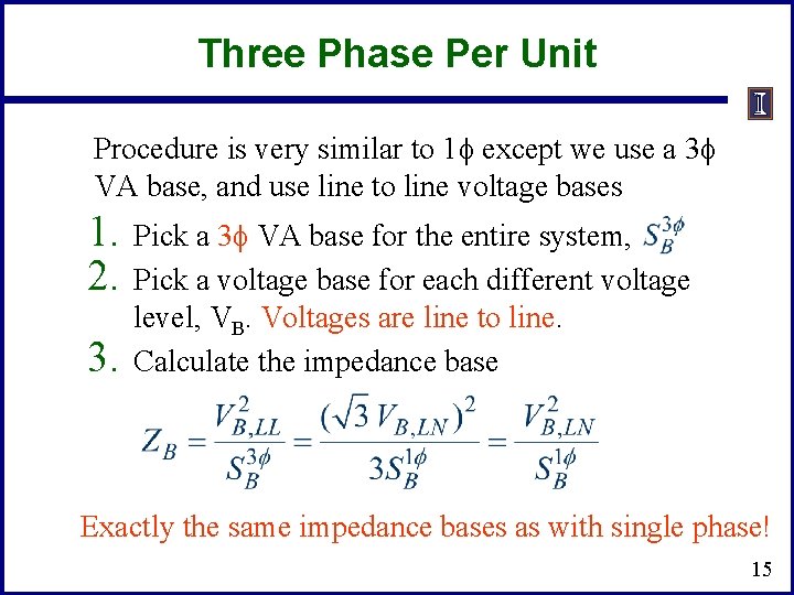
Three Phase Per Unit Procedure is very similar to 1 f except we use a 3 f VA base, and use line to line voltage bases 1. 2. 3. Pick a 3 f VA base for the entire system, Pick a voltage base for each different voltage level, VB. Voltages are line to line. Calculate the impedance base Exactly the same impedance bases as with single phase! 15

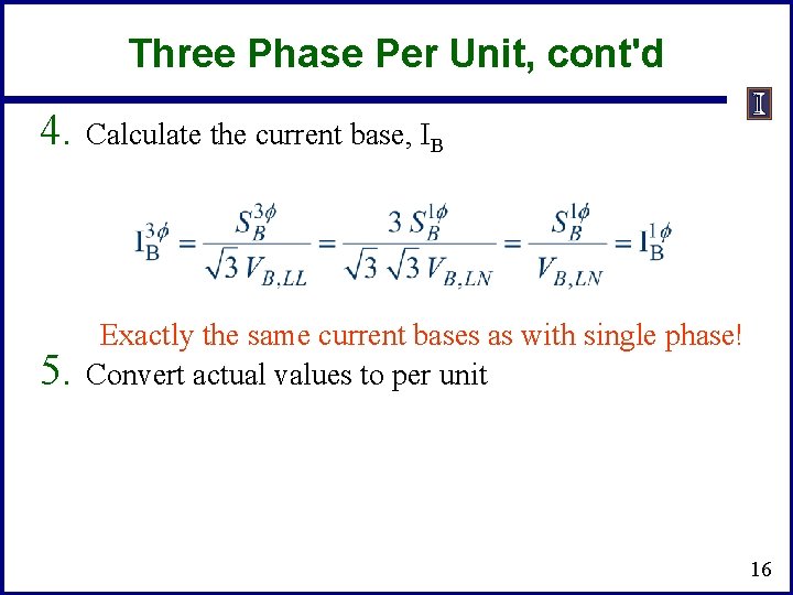
Three Phase Per Unit, cont'd 4. Calculate the current base, IB 5. Exactly the same current bases as with single phase! Convert actual values to per unit 16

Three Phase Per Unit Example Solve for the current, load voltage and load power in the previous circuit, assuming a 3 f power base of 300 MVA, and line to line voltage bases of 13. 8 k. V, 138 k. V and 27. 6 k. V (square root of 3 larger than the 1 f example voltages). Also assume the generator is Y -connected so its line to line voltage is 13. 8 k. V. Convert to per unit as before. Note the system is exactly the same! 17

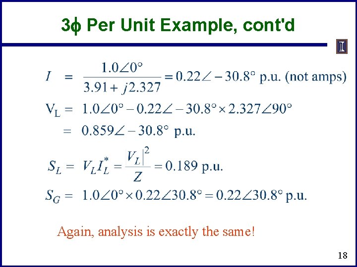
3 f Per Unit Example, cont'd Again, analysis is exactly the same! 18

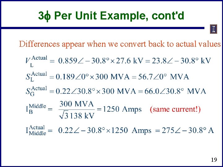
3 f Per Unit Example, cont'd Differences appear when we convert back to actual values 19

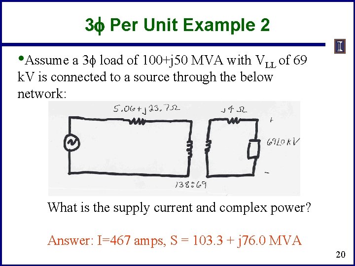
3 f Per Unit Example 2 • Assume a 3 f load of 100+j 50 MVA with VLL of 69 k. V is connected to a source through the below network: What is the supply current and complex power? Answer: I=467 amps, S = 103. 3 + j 76. 0 MVA 20

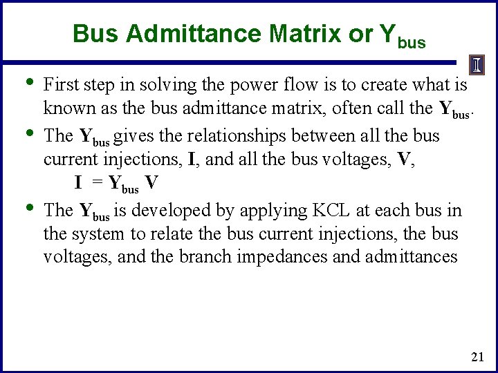
Bus Admittance Matrix or Ybus • • • First step in solving the power flow is to create what is known as the bus admittance matrix, often call the Ybus. The Ybus gives the relationships between all the bus current injections, I, and all the bus voltages, V, I = Ybus V The Ybus is developed by applying KCL at each bus in the system to relate the bus current injections, the bus voltages, and the branch impedances and admittances 21

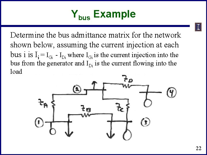
Ybus Example Determine the bus admittance matrix for the network shown below, assuming the current injection at each bus i is Ii = IGi - IDi where IGi is the current injection into the bus from the generator and IDi is the current flowing into the load 22

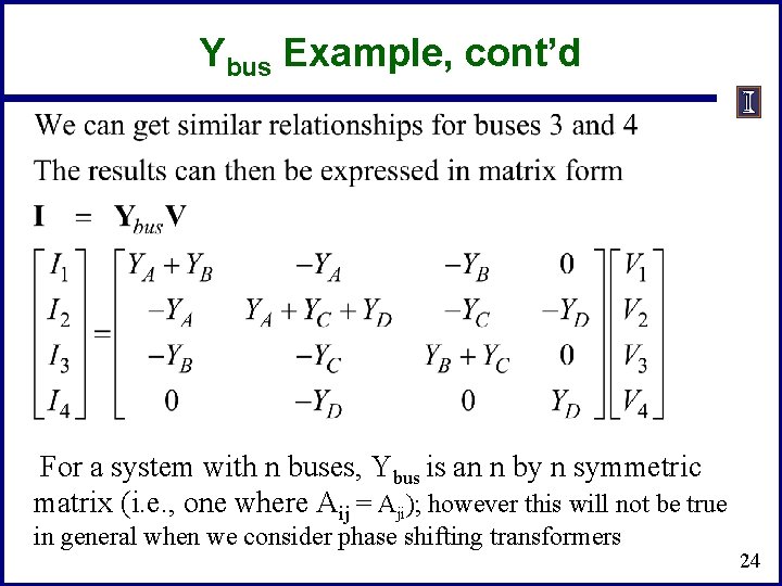
Ybus Example, cont’d = 23

Ybus Example, cont’d For a system with n buses, Ybus is an n by n symmetric matrix (i. e. , one where Aij = Aji); however this will not be true in general when we consider phase shifting transformers 24

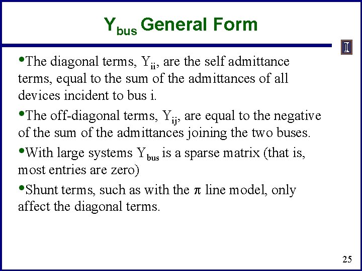
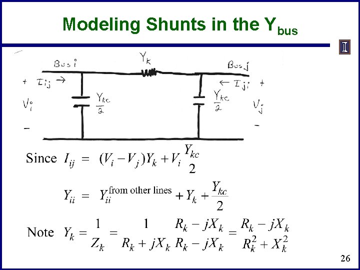
Ybus General Form • The diagonal terms, Yii, are the self admittance terms, equal to the sum of the admittances of all devices incident to bus i. • The off-diagonal terms, Yij, are equal to the negative of the sum of the admittances joining the two buses. • With large systems Ybus is a sparse matrix (that is, most entries are zero) • Shunt terms, such as with the p line model, only affect the diagonal terms. 25

Modeling Shunts in the Ybus 26

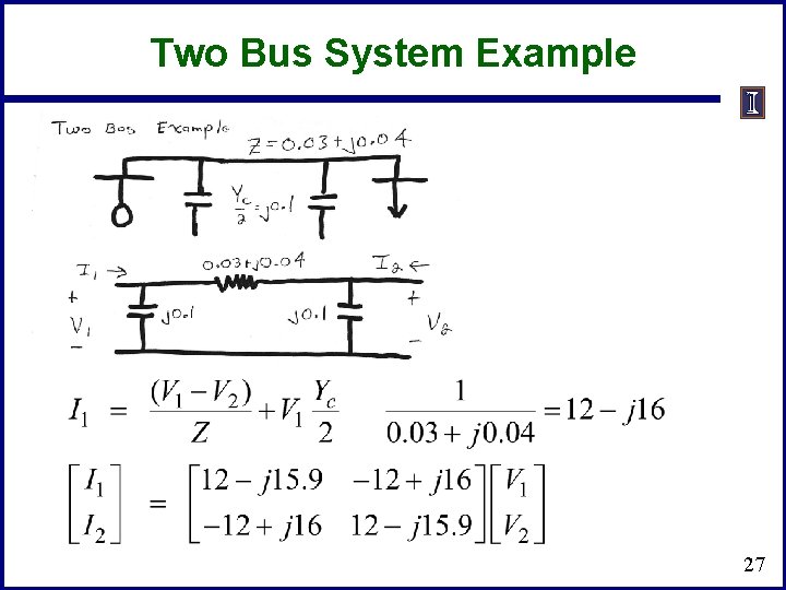
Two Bus System Example 27

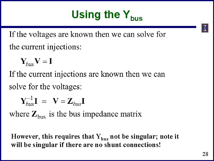
Using the Ybus However, this requires that Ybus not be singular; note it will be singular if there are no shunt connections! 28

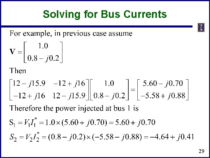
Solving for Bus Currents 29

Solving for Bus Voltages 30

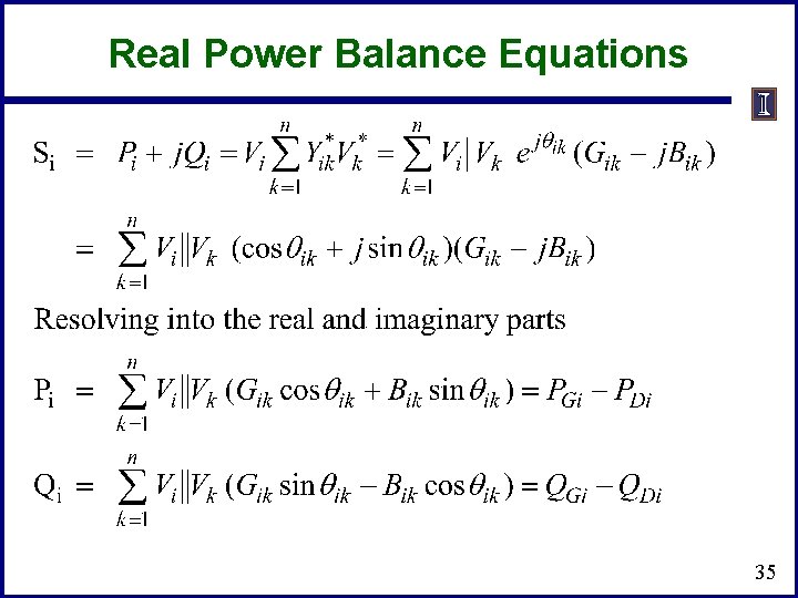
Power Flow Analysis • • • When analyzing power systems we know neither the complex bus voltages nor the complex current injections Rather, we know the complex power being consumed by the load, and the power being injected by the generators plus their voltage magnitudes Therefore we can not directly use the Ybus equations, but rather must use the power balance equations 31

Power Flow Analysis • • • Classic paper for this lecture is W. F. Tinney and C. E. Hart, “Power Flow Solution by Newton’s Method, ” IEEE Power App System, Nov 1967 Basic power flow is also covered in essentially power system analysis textbooks. At Illinois we use the term “power flow” not “load flow” since power flows not load. Also, the power flow usage is not new (see title of Tinney’s 1967 paper, and note Tinney references Ward’s 1956 paper) – A nice history of the power flow is given in an insert by Alvarado and Thomas in T. J. Overbye, J. D. Weber, “Visualizing the Electric Grid, ” IEEE Spectrum, Feb 2001. 32

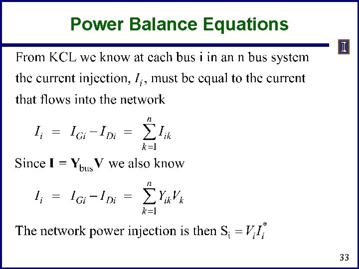
Power Balance Equations 33

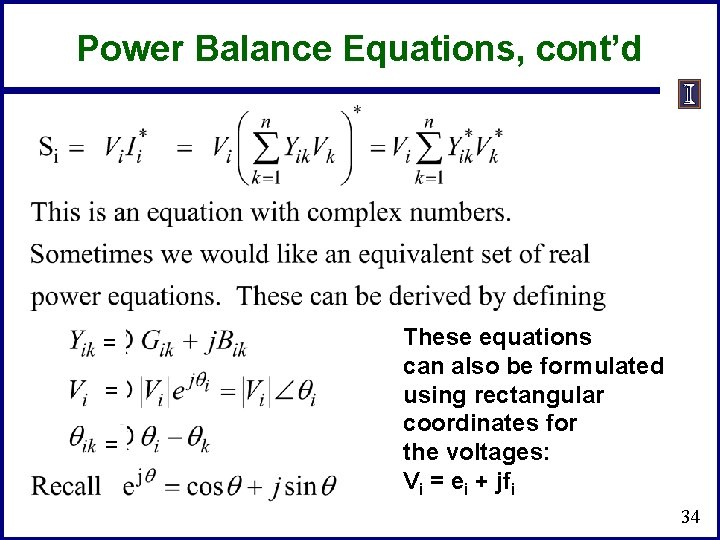
Power Balance Equations, cont’d = = = These equations can also be formulated using rectangular coordinates for the voltages: Vi = ei + jfi 34

Real Power Balance Equations 35

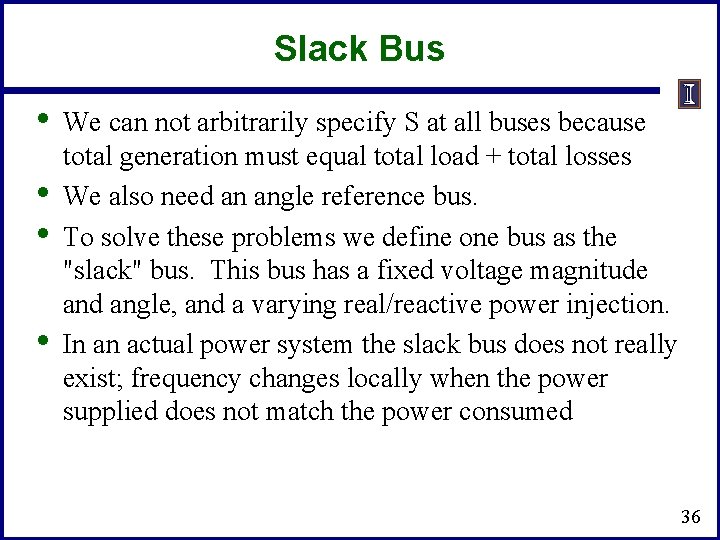
Slack Bus • • We can not arbitrarily specify S at all buses because total generation must equal total load + total losses We also need an angle reference bus. To solve these problems we define one bus as the "slack" bus. This bus has a fixed voltage magnitude and angle, and a varying real/reactive power injection. In an actual power system the slack bus does not really exist; frequency changes locally when the power supplied does not match the power consumed 36

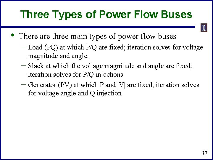
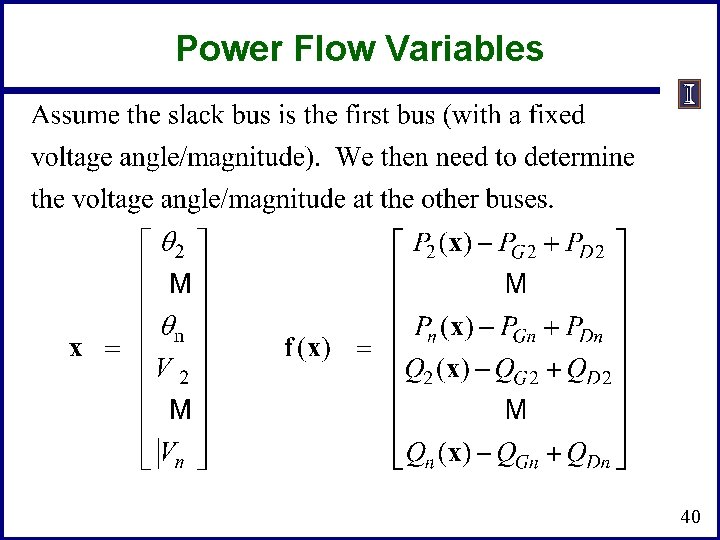
Three Types of Power Flow Buses • There are three main types of power flow buses – Load (PQ) at which P/Q are fixed; iteration solves for voltage magnitude and angle. – Slack at which the voltage magnitude and angle are fixed; iteration solves for P/Q injections – Generator (PV) at which P and |V| are fixed; iteration solves for voltage angle and Q injection 37

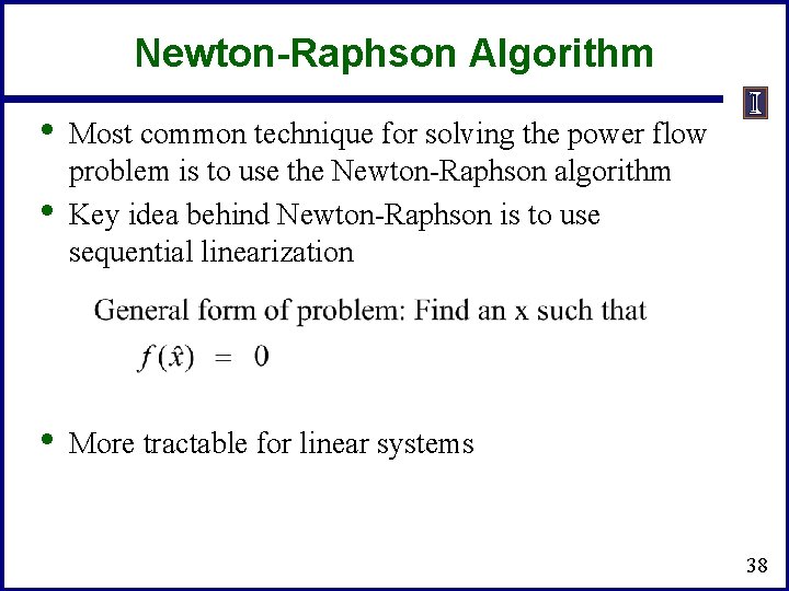
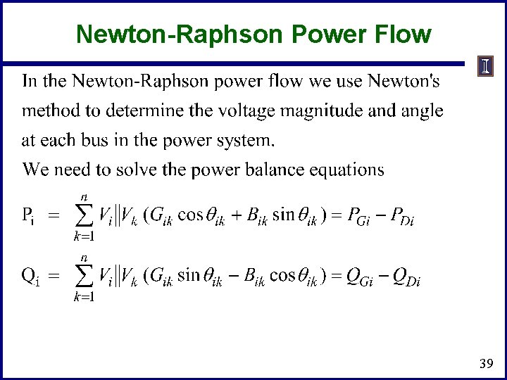
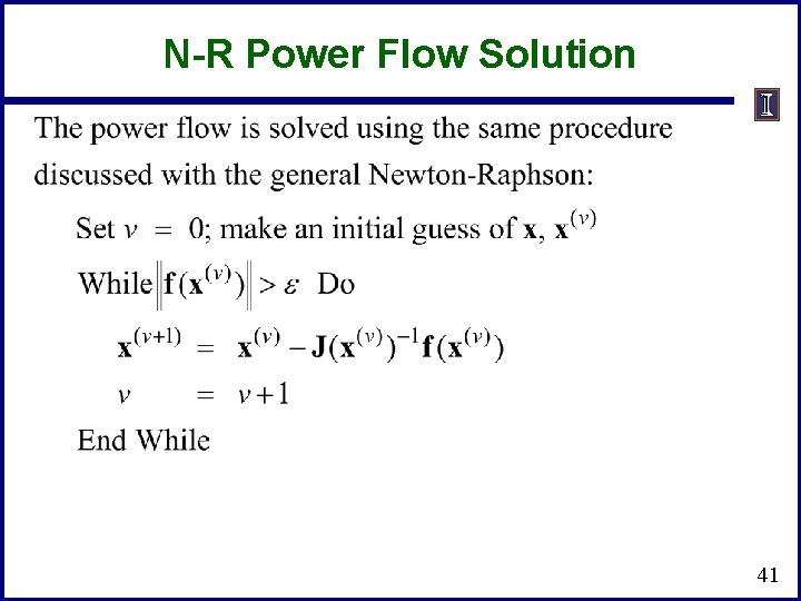
Newton-Raphson Algorithm • • • Most common technique for solving the power flow problem is to use the Newton-Raphson algorithm Key idea behind Newton-Raphson is to use sequential linearization More tractable for linear systems 38

Newton-Raphson Power Flow 39

Power Flow Variables 40

N-R Power Flow Solution 41

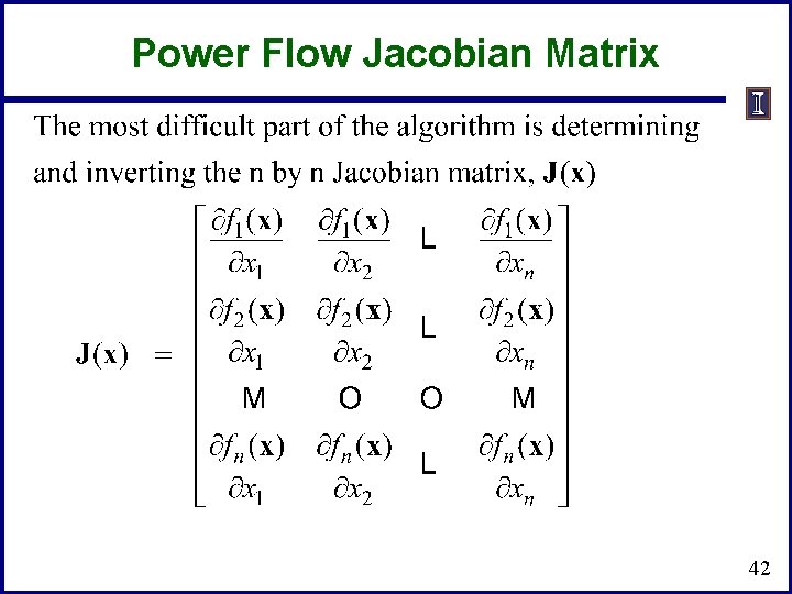
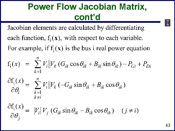
Power Flow Jacobian Matrix 42

Power Flow Jacobian Matrix, cont’d 43