1 CE 530 Molecular Simulation Lecture 22 ChainMolecule



- Slides: 35

1 CE 530 Molecular Simulation Lecture 22 Chain-Molecule Sampling Techniques David A. Kofke Department of Chemical Engineering SUNY Buffalo kofke@eng. buffalo. edu

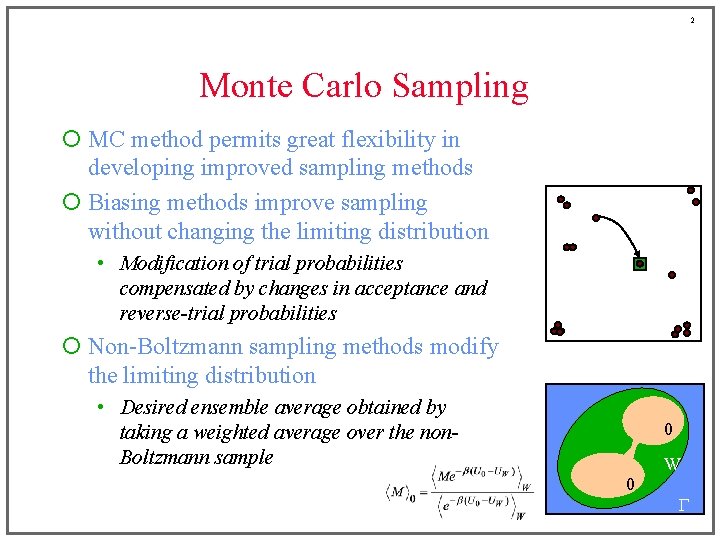
2 Monte Carlo Sampling ¡ MC method permits great flexibility in developing improved sampling methods ¡ Biasing methods improve sampling without changing the limiting distribution • Modification of trial probabilities compensated by changes in acceptance and reverse-trial probabilities ¡ Non-Boltzmann sampling methods modify the limiting distribution • Desired ensemble average obtained by taking a weighted average over the non. Boltzmann sample 0 W 0 G

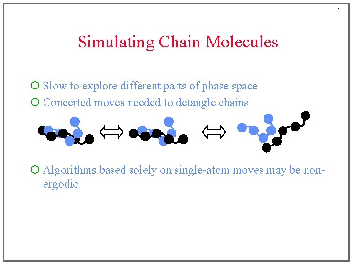
3 Simulating Chain Molecules ¡ Slow to explore different parts of phase space ¡ Concerted moves needed to detangle chains ¡ Algorithms based solely on single-atom moves may be nonergodic

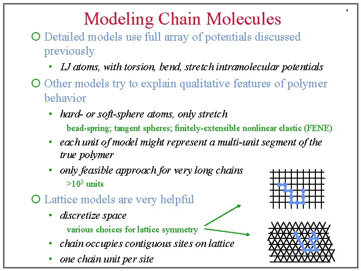
Modeling Chain Molecules ¡ Detailed models use full array of potentials discussed previously • LJ atoms, with torsion, bend, stretch intramolecular potentials ¡ Other models try to explain qualitative features of polymer behavior • hard- or soft-sphere atoms, only stretch bead-spring; tangent spheres; finitely-extensible nonlinear elastic (FENE) • each unit of model might represent a multi-unit segment of the true polymer • only feasible approach for very long chains >103 units ¡ Lattice models are very helpful • discretize space various choices for lattice symmetry • chain occupies contiguous sites on lattice • one chain unit per site 4

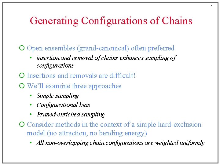
5 Generating Configurations of Chains ¡ Open ensembles (grand-canonical) often preferred • insertion and removal of chains enhances sampling of configurations ¡ Insertions and removals are difficult! ¡ We’ll examine three approaches • Simple sampling • Configurational bias • Pruned-enriched sampling ¡ Consider methods in the context of a simple hard-exclusion model (no attraction, no bending energy) • All non-overlapping chain configurations are weighted uniformly

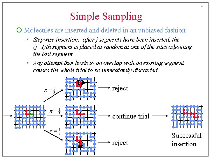
6 Simple Sampling ¡ Molecules are inserted and deleted in an unbiased fashion • Stepwise insertion: after j segments have been inserted, the (j+1)th segment is placed at random at one of the sites adjoining the last segment • Any attempt that leads to an overlap with an existing segment causes the whole trial to be immediately discarded reject continue trial reject Successful insertion

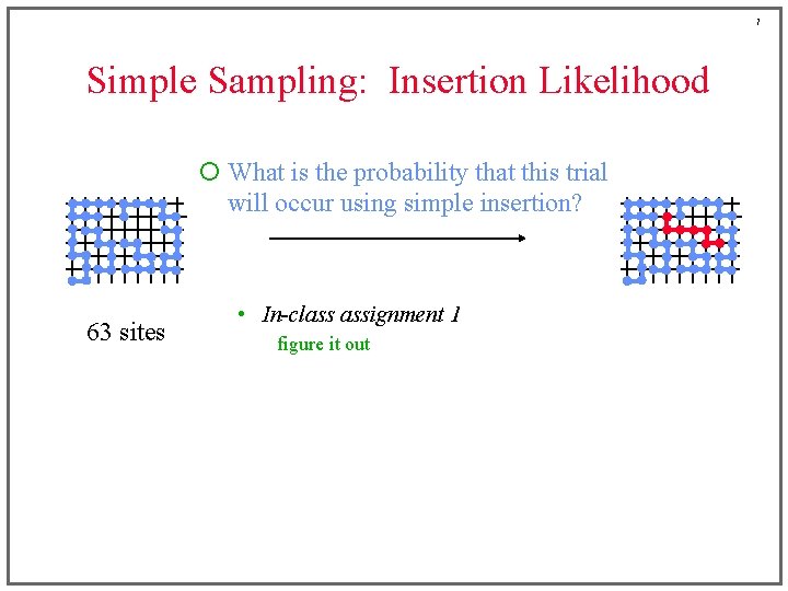
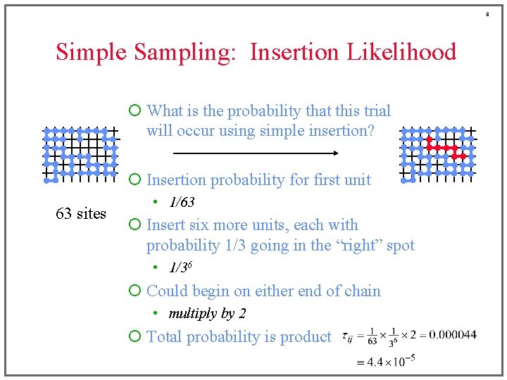
7 Simple Sampling: Insertion Likelihood ¡ What is the probability that this trial will occur using simple insertion? 63 sites • In-class assignment 1 figure it out

8 Simple Sampling: Insertion Likelihood ¡ What is the probability that this trial will occur using simple insertion? ¡ Insertion probability for first unit 63 sites • 1/63 ¡ Insert six more units, each with probability 1/3 going in the “right” spot • 1/36 ¡ Could begin on either end of chain • multiply by 2 ¡ Total probability is product

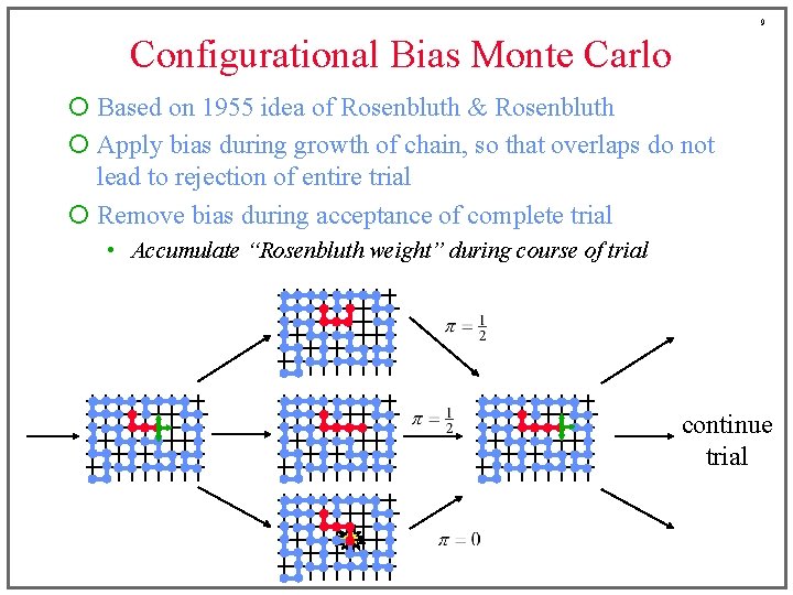
9 Configurational Bias Monte Carlo ¡ Based on 1955 idea of Rosenbluth & Rosenbluth ¡ Apply bias during growth of chain, so that overlaps do not lead to rejection of entire trial ¡ Remove bias during acceptance of complete trial • Accumulate “Rosenbluth weight” during course of trial continue trial

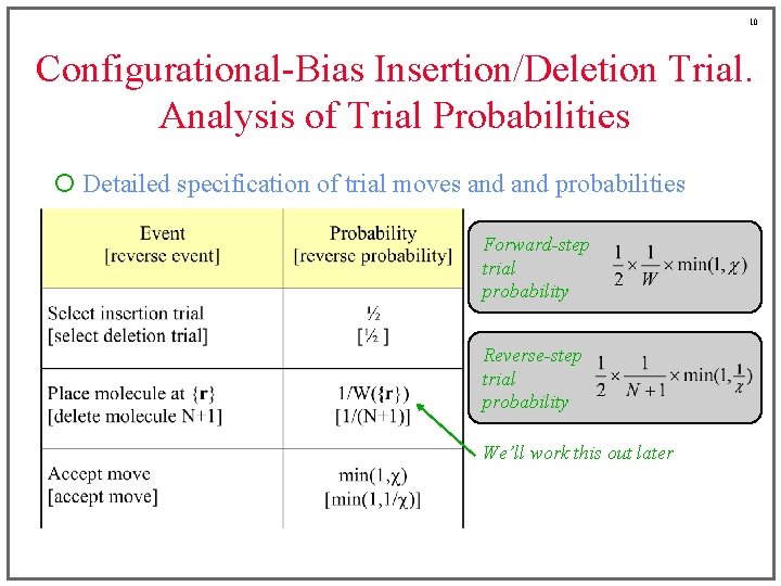
10 Configurational-Bias Insertion/Deletion Trial. Analysis of Trial Probabilities ¡ Detailed specification of trial moves and probabilities Forward-step trial probability Reverse-step trial probability We’ll work this out later

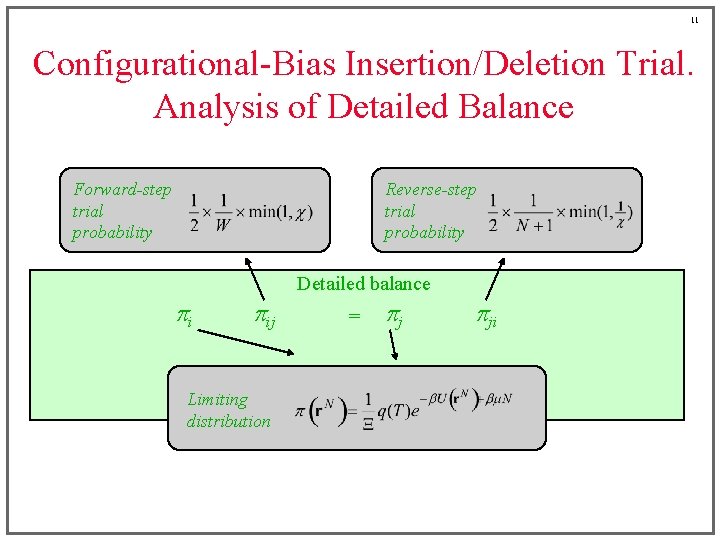
11 Configurational-Bias Insertion/Deletion Trial. Analysis of Detailed Balance Forward-step trial probability Reverse-step trial probability Detailed balance pi pij Limiting distribution = pj pji

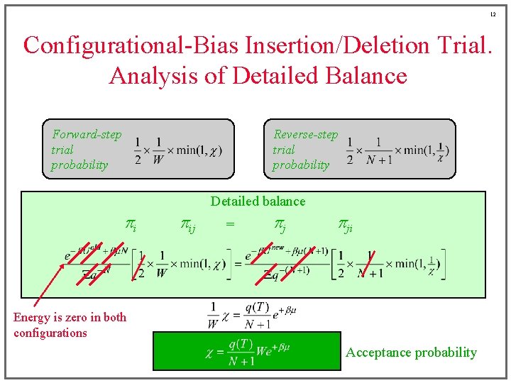
12 Configurational-Bias Insertion/Deletion Trial. Analysis of Detailed Balance Forward-step trial probability Reverse-step trial probability Detailed balance pi pij = pj pji Energy is zero in both configurations Acceptance probability

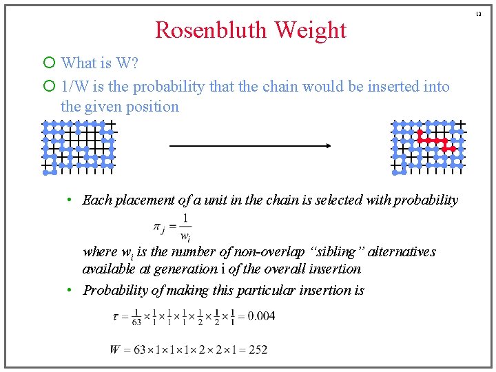
Rosenbluth Weight ¡ What is W? ¡ 1/W is the probability that the chain would be inserted into the given position • Each placement of a unit in the chain is selected with probability where wi is the number of non-overlap “sibling” alternatives available at generation i of the overall insertion • Probability of making this particular insertion is 13

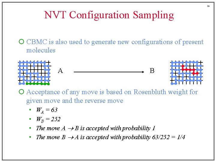
14 NVT Configuration Sampling ¡ CBMC is also used to generate new configurations of present molecules A B ¡ Acceptance of any move is based on Rosenbluth weight for given move and the reverse move • • WA = 63 WB = 252 The move A B is accepted with probability 1 The move B A is accepted with probability 63/252 = 1/4

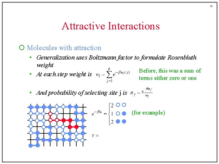
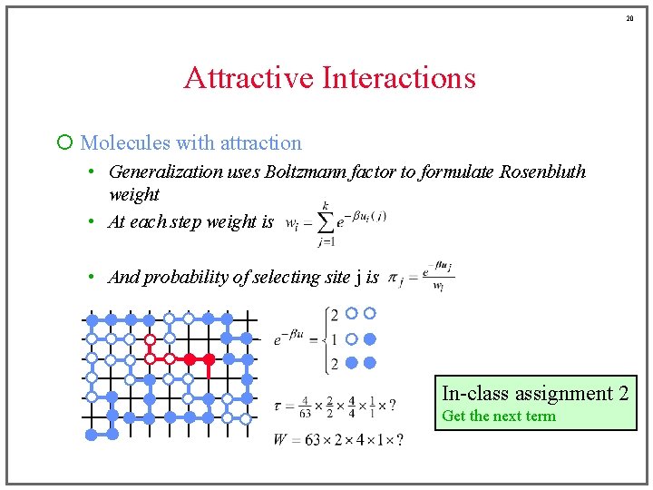
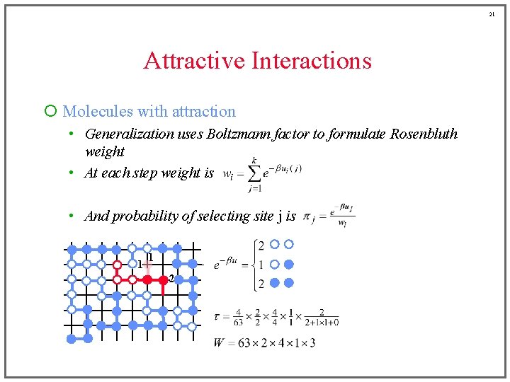
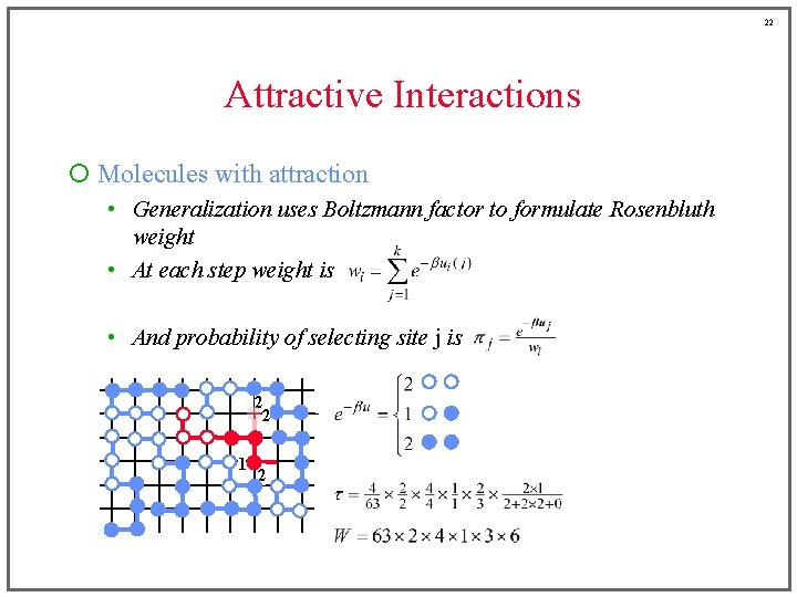
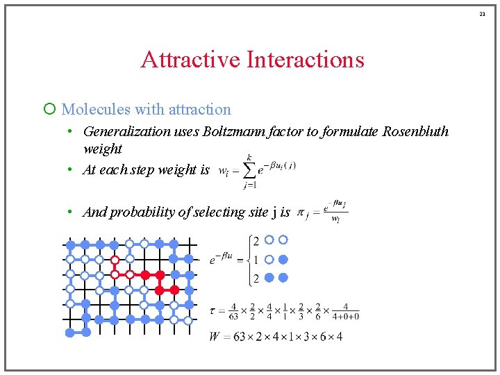
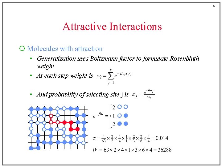
15 Attractive Interactions ¡ Molecules with attraction • Generalization uses Boltzmann factor to formulate Rosenbluth weight Before, this was a sum of • At each step weight is terms either zero or one • And probability of selecting site j is (for example)

16 Attractive Interactions ¡ Molecules with attraction • Generalization uses Boltzmann factor to formulate Rosenbluth weight • At each step weight is • And probability of selecting site j is 1 2 2

17 Attractive Interactions ¡ Molecules with attraction • Generalization uses Boltzmann factor to formulate Rosenbluth weight • At each step weight is • And probability of selecting site j is 2 1

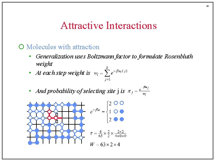
18 Attractive Interactions ¡ Molecules with attraction • Generalization uses Boltzmann factor to formulate Rosenbluth weight • At each step weight is • And probability of selecting site j is 2 2

19 Attractive Interactions ¡ Molecules with attraction • Generalization uses Boltzmann factor to formulate Rosenbluth weight • At each step weight is • And probability of selecting site j is 1

20 Attractive Interactions ¡ Molecules with attraction • Generalization uses Boltzmann factor to formulate Rosenbluth weight • At each step weight is • And probability of selecting site j is In-class assignment 2 Get the next term

21 Attractive Interactions ¡ Molecules with attraction • Generalization uses Boltzmann factor to formulate Rosenbluth weight • At each step weight is • And probability of selecting site j is 1 1 2

22 Attractive Interactions ¡ Molecules with attraction • Generalization uses Boltzmann factor to formulate Rosenbluth weight • At each step weight is • And probability of selecting site j is 2 2 1 2

23 Attractive Interactions ¡ Molecules with attraction • Generalization uses Boltzmann factor to formulate Rosenbluth weight • At each step weight is • And probability of selecting site j is

24 Attractive Interactions ¡ Molecules with attraction • Generalization uses Boltzmann factor to formulate Rosenbluth weight • At each step weight is • And probability of selecting site j is

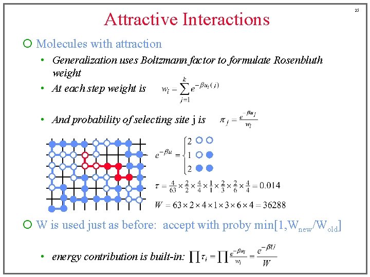
Attractive Interactions ¡ Molecules with attraction • Generalization uses Boltzmann factor to formulate Rosenbluth weight • At each step weight is • And probability of selecting site j is ¡ W is used just as before: accept with proby min[1, Wnew/Wold] • energy contribution is built-in: 25

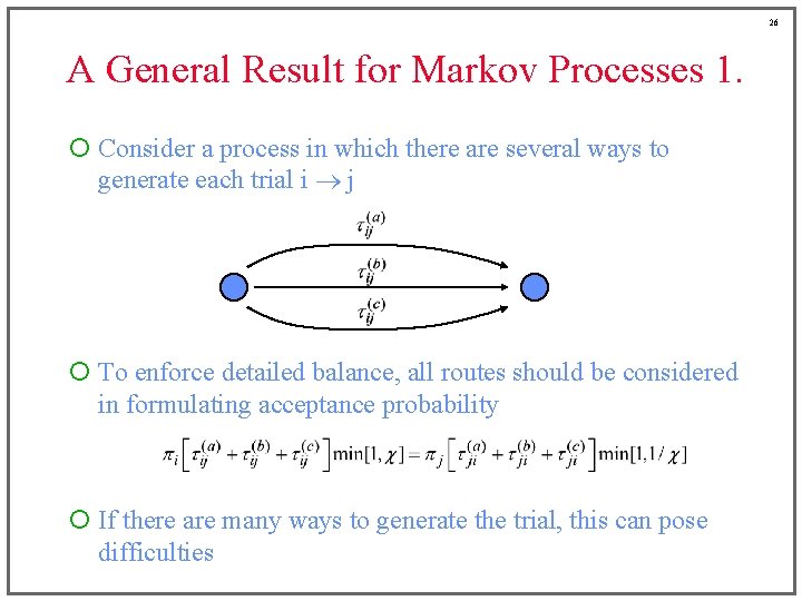
26 A General Result for Markov Processes 1. ¡ Consider a process in which there are several ways to generate each trial i j ¡ To enforce detailed balance, all routes should be considered in formulating acceptance probability ¡ If there are many ways to generate the trial, this can pose difficulties

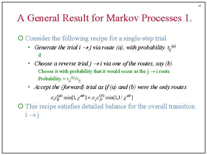
27 A General Result for Markov Processes 1. ¡ Consider the following recipe for a single-step trial • Generate the trial i j via route (a), with probability tij(a) d • Choose a reverse trial j i via one of the routes, say (b) Choose it with probability that it would occur as the j i route Probability = tji(b)/tji • Accept the (forward) trial as if (a) and (b) were the only routes ¡ This recipe satisfies detailed balance for the overall transition i j

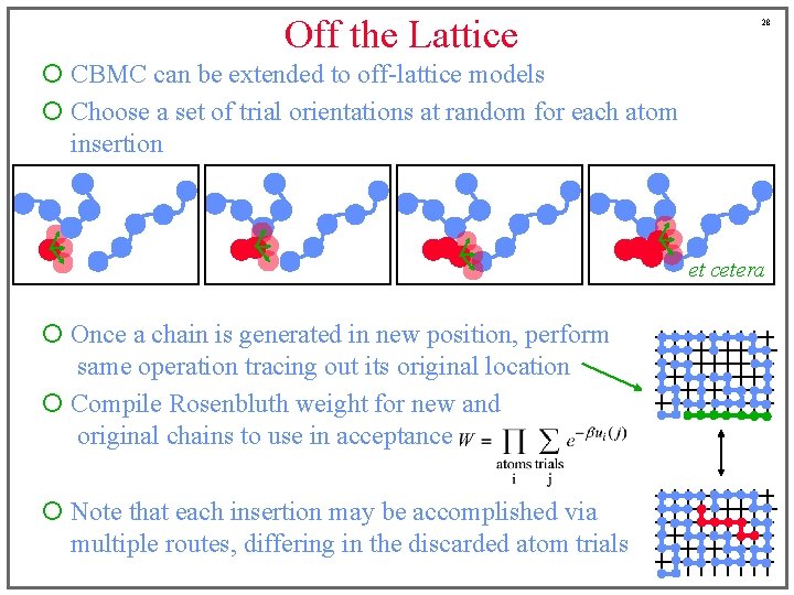
Off the Lattice 28 ¡ CBMC can be extended to off-lattice models ¡ Choose a set of trial orientations at random for each atom insertion et cetera ¡ Once a chain is generated in new position, perform same operation tracing out its original location ¡ Compile Rosenbluth weight for new and original chains to use in acceptance ¡ Note that each insertion may be accomplished via multiple routes, differing in the discarded atom trials

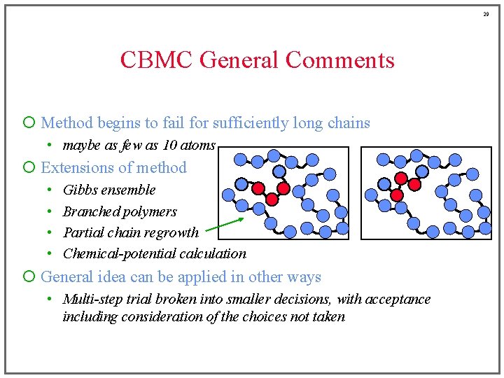
29 CBMC General Comments ¡ Method begins to fail for sufficiently long chains • maybe as few as 10 atoms ¡ Extensions of method • • Gibbs ensemble Branched polymers Partial chain regrowth Chemical-potential calculation ¡ General idea can be applied in other ways • Multi-step trial broken into smaller decisions, with acceptance including consideration of the choices not taken

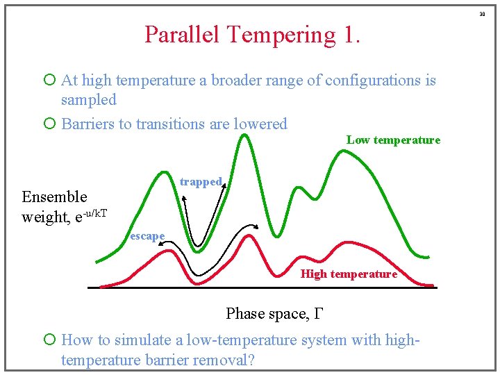
30 Parallel Tempering 1. ¡ At high temperature a broader range of configurations is sampled ¡ Barriers to transitions are lowered Low temperature trapped Ensemble weight, e-u/k. T escape High temperature Phase space, G ¡ How to simulate a low-temperature system with hightemperature barrier removal?

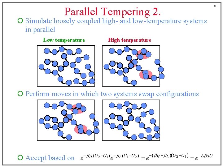
Parallel Tempering 2. ¡ Simulate loosely coupled high- and low-temperature systems in parallel Low temperature High temperature ¡ Perform moves in which two systems swap configurations ¡ Accept based on 31

32 Parallel Tempering 3. ¡ To get reasonable acceptance rate, temperatures should not be too different ¡ Can be extended to include any number of systems simulated in parallel ¡ Can be extended to do “tempering” in other variables, such as the chemical potential ¡ Very well suited for use in conjunction with histogram reweighting

33 Pruned-Enriched Rosenbluth Method ¡ At some point along the growth process it may become clear that • the chain is doomed, or • the chain is really doing well ¡ We’d like to enrich the presence of the good ones, while pruning out the ones that look bad ¡ Use a criterion based on partial Rosenbluth weight

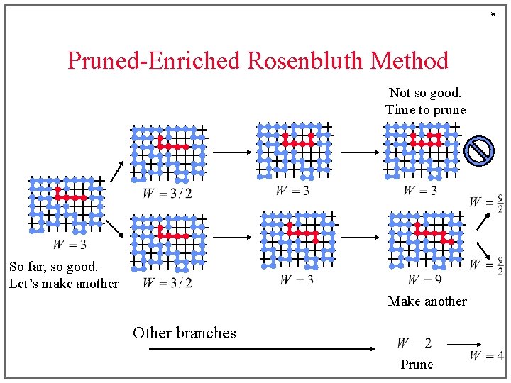
34 Pruned-Enriched Rosenbluth Method Not so good. Time to prune So far, so good. Let’s make another Make another Other branches Prune

35 Pruned-Enriched Rosenbluth Method ¡ Set cutoffs for intermediate Rosenbluth weights • duplicate any configuration having W > W>, halving weights of new duplicates • prune configurations having W < W<, taking every-other such configuration, and doubling the weight of those not taken