1 CE 530 Molecular Simulation Lecture 3 David
- Slides: 17

1 CE 530 Molecular Simulation Lecture 3 David A. Kofke Department of Chemical Engineering SUNY Buffalo kofke@eng. buffalo. edu

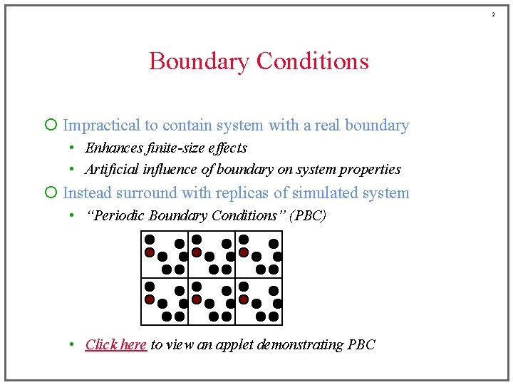
2 Boundary Conditions ¡ Impractical to contain system with a real boundary • Enhances finite-size effects • Artificial influence of boundary on system properties ¡ Instead surround with replicas of simulated system • “Periodic Boundary Conditions” (PBC) • Click here to view an applet demonstrating PBC

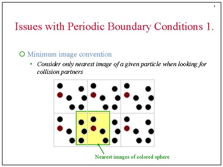
3 Issues with Periodic Boundary Conditions 1. ¡ Minimum image convention • Consider only nearest image of a given particle when looking for collision partners Nearest images of colored sphere

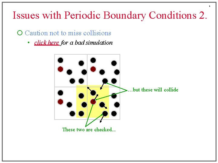
4 Issues with Periodic Boundary Conditions 2. ¡ Caution not to miss collisions • click here for a bad simulation …but these will collide These two are checked. . .

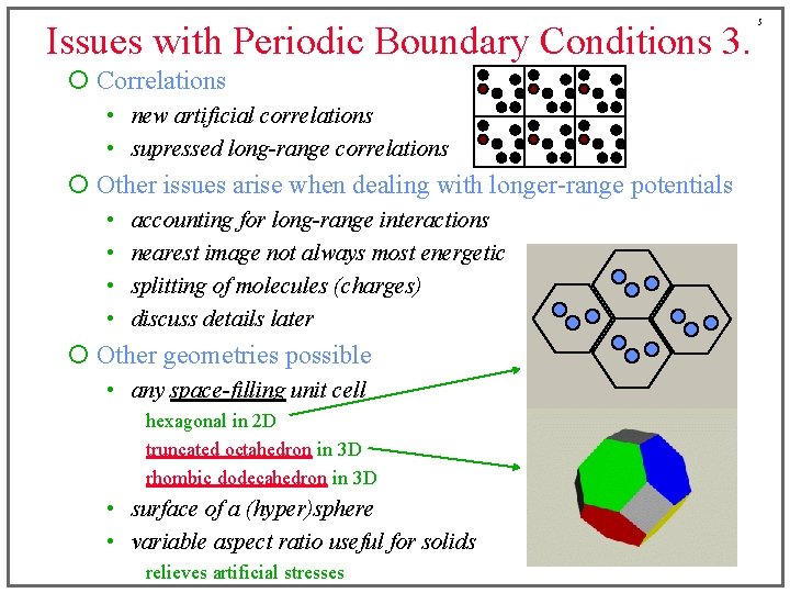
Issues with Periodic Boundary Conditions 3. ¡ Correlations • new artificial correlations • supressed long-range correlations ¡ Other issues arise when dealing with longer-range potentials • • accounting for long-range interactions nearest image not always most energetic splitting of molecules (charges) discuss details later ¡ Other geometries possible • any space-filling unit cell hexagonal in 2 D truncated octahedron in 3 D rhombic dodecahedron in 3 D • surface of a (hyper)sphere • variable aspect ratio useful for solids relieves artificial stresses 5

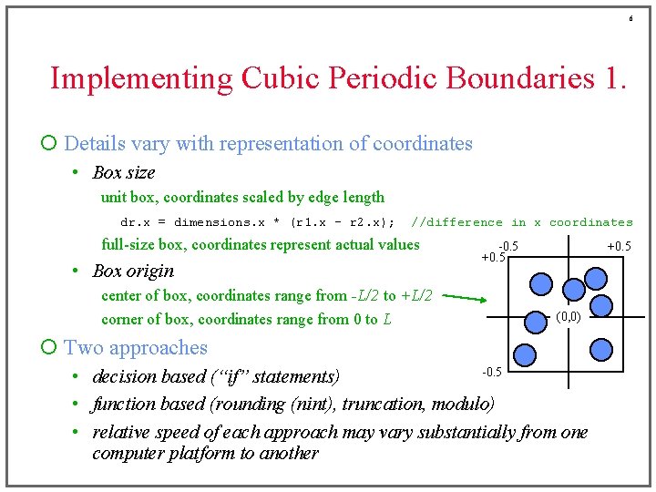
6 Implementing Cubic Periodic Boundaries 1. ¡ Details vary with representation of coordinates • Box size unit box, coordinates scaled by edge length dr. x = dimensions. x * (r 1. x - r 2. x); //difference in x coordinates full-size box, coordinates represent actual values • Box origin center of box, coordinates range from -L/2 to +L/2 corner of box, coordinates range from 0 to L -0. 5 +0. 5 (0, 0) ¡ Two approaches -0. 5 • decision based (“if” statements) • function based (rounding (nint), truncation, modulo) • relative speed of each approach may vary substantially from one computer platform to another

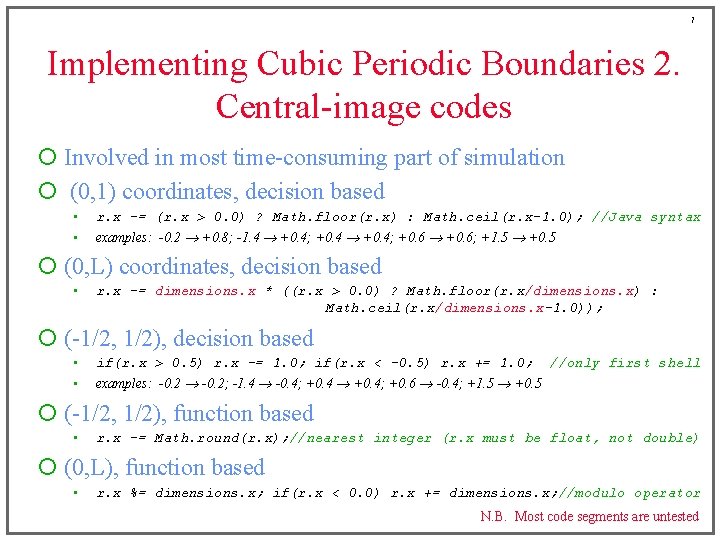
7 Implementing Cubic Periodic Boundaries 2. Central-image codes ¡ Involved in most time-consuming part of simulation ¡ (0, 1) coordinates, decision based • • r. x -= (r. x > 0. 0) ? Math. floor(r. x) : Math. ceil(r. x-1. 0); //Java syntax examples: -0. 2 +0. 8; -1. 4 +0. 4; +0. 6; +1. 5 +0. 5 ¡ (0, L) coordinates, decision based • r. x -= dimensions. x * ((r. x > 0. 0) ? Math. floor(r. x/dimensions. x) : Math. ceil(r. x/dimensions. x-1. 0)); ¡ (-1/2, 1/2), decision based • • if(r. x > 0. 5) r. x -= 1. 0; if(r. x < -0. 5) r. x += 1. 0; //only first shell examples: -0. 2; -1. 4 -0. 4; +0. 6 -0. 4; +1. 5 +0. 5 ¡ (-1/2, 1/2), function based • r. x -= Math. round(r. x); //nearest integer (r. x must be float, not double) ¡ (0, L), function based • r. x %= dimensions. x; if(r. x < 0. 0) r. x += dimensions. x; //modulo operator N. B. Most code segments are untested

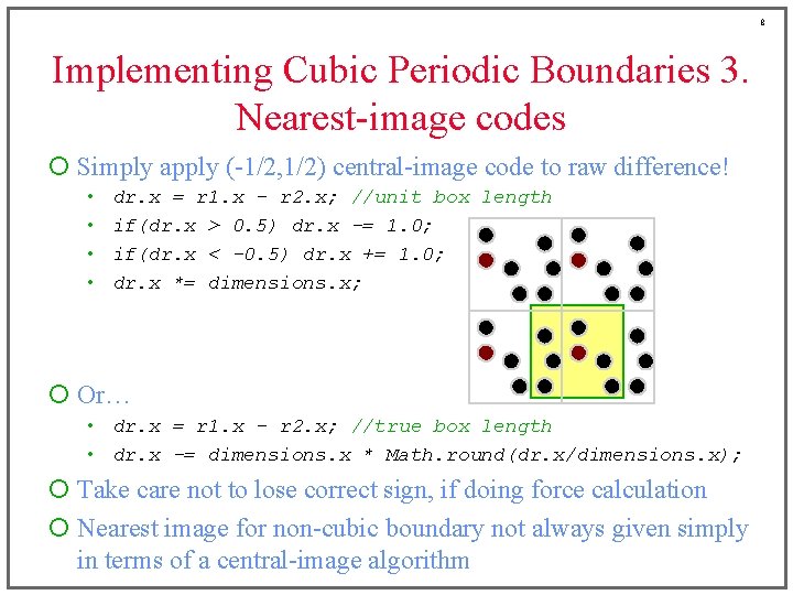
8 Implementing Cubic Periodic Boundaries 3. Nearest-image codes ¡ Simply apply (-1/2, 1/2) central-image code to raw difference! • • dr. x = r 1. x - r 2. x; //unit box length if(dr. x > 0. 5) dr. x -= 1. 0; if(dr. x < -0. 5) dr. x += 1. 0; dr. x *= dimensions. x; ¡ Or… • dr. x = r 1. x - r 2. x; //true box length • dr. x -= dimensions. x * Math. round(dr. x/dimensions. x); ¡ Take care not to lose correct sign, if doing force calculation ¡ Nearest image for non-cubic boundary not always given simply in terms of a central-image algorithm

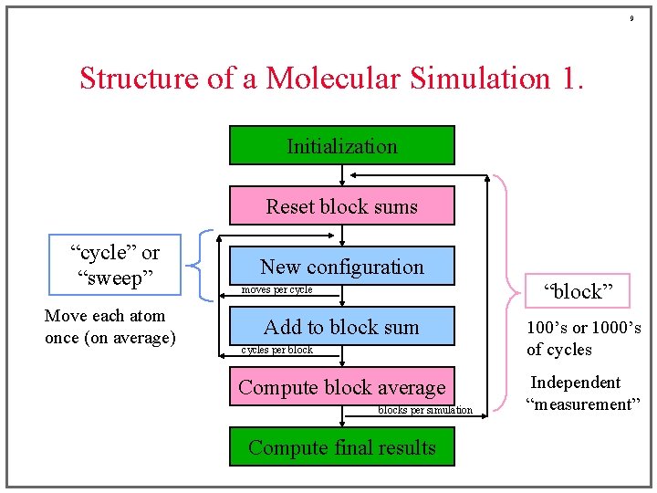
9 Structure of a Molecular Simulation 1. Initialization Reset block sums “cycle” or “sweep” Move each atom once (on average) New configuration “block” moves per cycle Add to block sum cycles per block Compute block average blocks per simulation Compute final results 100’s or 1000’s of cycles Independent “measurement”

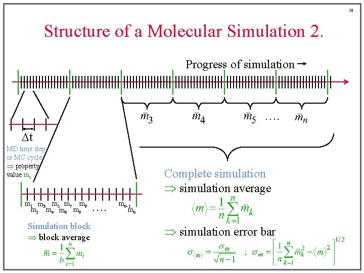
10 Structure of a Molecular Simulation 2. Progress of simulation …. Dt MD time step or MC cycle property value mi m 1 m 3 m 5 m 7 m 9 m 2 m 4 m 6 m 8 Simulation block average Complete simulation average …. mb-1 mb simulation error bar

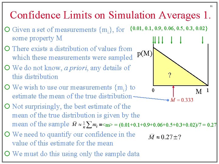
11 Confidence Limits on Simulation Averages 1. ¡ Given a set of measurements {mi}, for {0. 01, 0. 9, 0. 06, 0. 5, 0. 3, 0. 02} some property M ¡ There exists a distribution of values from p(M) which these measurements were sampled ¡ We do not know, a priori, any details of ? this distribution ¡ We wish to use our measurements {mi} to 0 M 1 estimate the mean of the true distribution ¡ Not surprisingly, the best estimate of the mean of the true distribution is given by the mean of the sample <m> = (0. 01+0. 9+0. 06+0. 5+0. 3+0. 02)/7 = 0. 27 ¡ We need to quantify our confidence in the value of this estimate for the mean ¡ We must do this using only the sample data

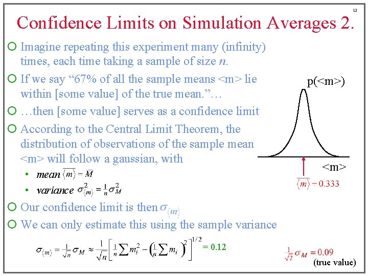
12 Confidence Limits on Simulation Averages 2. ¡ Imagine repeating this experiment many (infinity) times, each time taking a sample of size n. ¡ If we say “ 67% of all the sample means <m> lie within [some value] of the true mean. ”… ¡ …then [some value] serves as a confidence limit ¡ According to the Central Limit Theorem, the distribution of observations of the sample mean <m> will follow a gaussian, with • mean • variance p(<m>) <m> ¡ Our confidence limit is then ¡ We can only estimate this using the sample variance = 0. 12 (true value)

13 Confidence Limits on Simulation Averages 3. ¡ Expression for confidence limit (error bar) assumes independent samples • successive configurations in a simulation are (usually) not independent • block averages are independent for “sufficiently large” blocks ¡ Often 2 s is used for error bar (95% confidence interval) • when reporting error bars it is good practice to state definition ¡ Confidence limits quantify only statistical errors. Sometimes other sources of error are more significant • systematic errors poor sampling (non-ergodic) finite-size effects insufficient equilibration • programming errors • conceptual errors • limitations of the molecular model

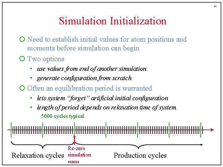
14 Simulation Initialization ¡ Need to establish initial values for atom positions and momenta before simulation can begin ¡ Two options • use values from end of another simulation • generate configuration from scratch ¡ Often an equilibration period is warranted • lets system “forget” artificial initial configuration • length of period depends on relaxation time of system 5000 cycles typical Relaxation cycles Re-zero simulation sums Production cycles

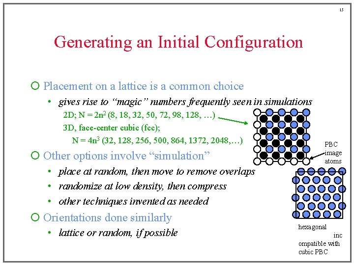
15 Generating an Initial Configuration ¡ Placement on a lattice is a common choice • gives rise to “magic” numbers frequently seen in simulations 2 D; N = 2 n 2 (8, 18, 32, 50, 72, 98, 128, …) 3 D, face-center cubic (fcc); N = 4 n 3 (32, 128, 256, 500, 864, 1372, 2048, …) ¡ Other options involve “simulation” PBC image atoms • place at random, then move to remove overlaps • randomize at low density, then compress • other techniques invented as needed ¡ Orientations done similarly • lattice or random, if possible hexagonal inc ompatible with cubic PBC

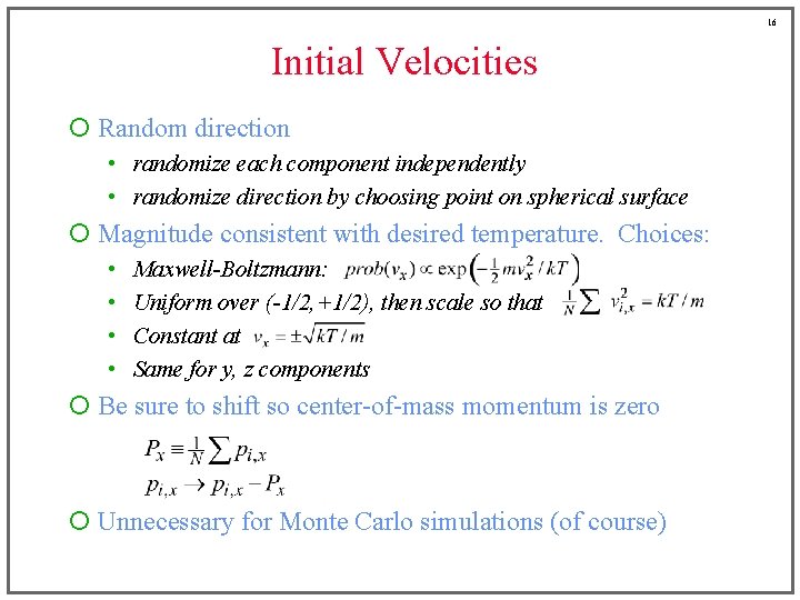
16 Initial Velocities ¡ Random direction • randomize each component independently • randomize direction by choosing point on spherical surface ¡ Magnitude consistent with desired temperature. Choices: • • Maxwell-Boltzmann: Uniform over (-1/2, +1/2), then scale so that Constant at Same for y, z components ¡ Be sure to shift so center-of-mass momentum is zero ¡ Unnecessary for Monte Carlo simulations (of course)

17 Summary of Simulation Elements ¡ Specification of state ¡ Units and dimensions, scaling ¡ Initialization ¡ Generation of configurations ¡ Property measurement ¡ Confidence limits ¡ Cycles and blocks ¡ Periodic boundaries ¡ Organizing and cycling through atom lists