ECE 530 Analysis Techniques for LargeScale Electrical Systems

ECE 530 – Analysis Techniques for Large-Scale Electrical Systems Lecture 25: A Primer on Dynamics & Stability Hao Zhu Dept. of Electrical and Computer Engineering University of Illinois at Urbana-Champaign haozhu@illinois. edu 12/7/2015 1

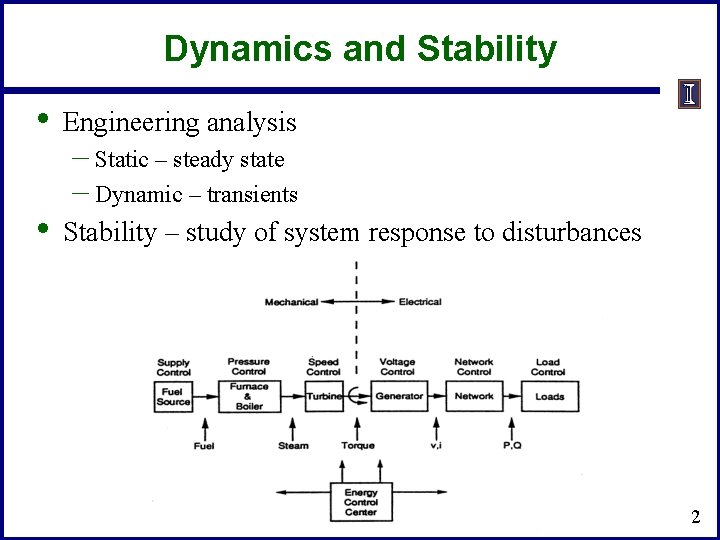
Dynamics and Stability • Engineering analysis • Stability – study of system response to disturbances – Static – steady state – Dynamic – transients 2

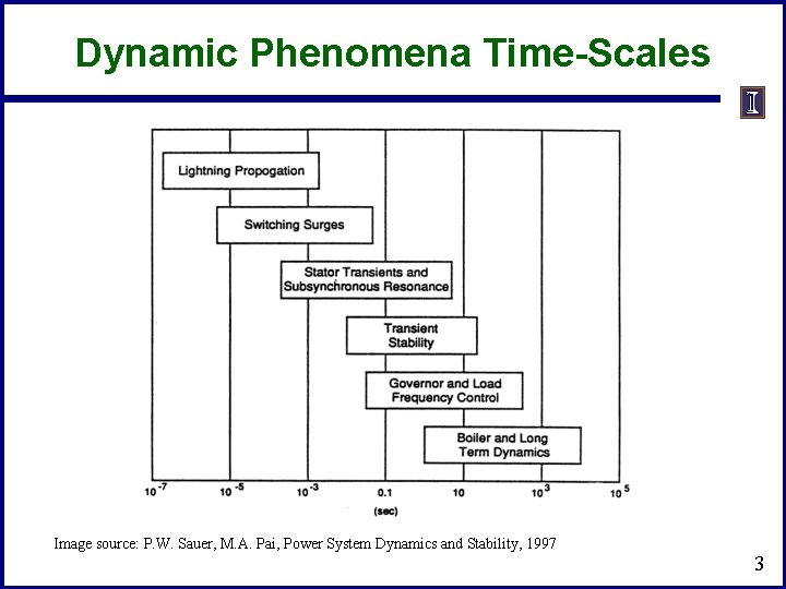
Dynamic Phenomena Time-Scales Image source: P. W. Sauer, M. A. Pai, Power System Dynamics and Stability, 1997 3

Transient Stability Analysis • • Time-scale of TS spans from sub-seconds to seconds This requires to consider the synchronization or asynchronization of multiple generators in interconnected areas We will first look at how to construct a set of differential algebraic equations (DAEs) for TS analysis A typical balancing authority (BA) area can be modeled with over 1000 diff. equations and 10, 000 algebraic constraint equations => Model-order reduction (MOR) or equivalencing is needed. 4

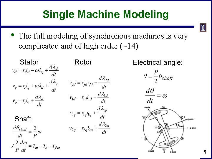
Single Machine Modeling • The full modeling of synchronous machines is very complicated and of high order (~14) Stator Rotor Electrical angle: Shaft 5

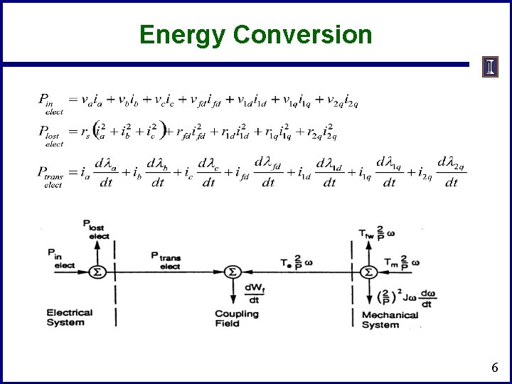
Energy Conversion 6

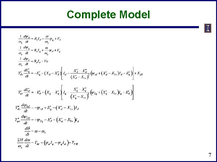
Complete Model 7

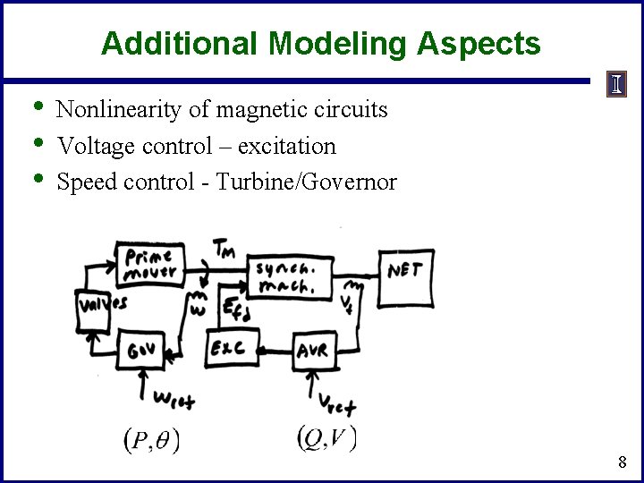
Additional Modeling Aspects • • • Nonlinearity of magnetic circuits Voltage control – excitation Speed control - Turbine/Governor 8

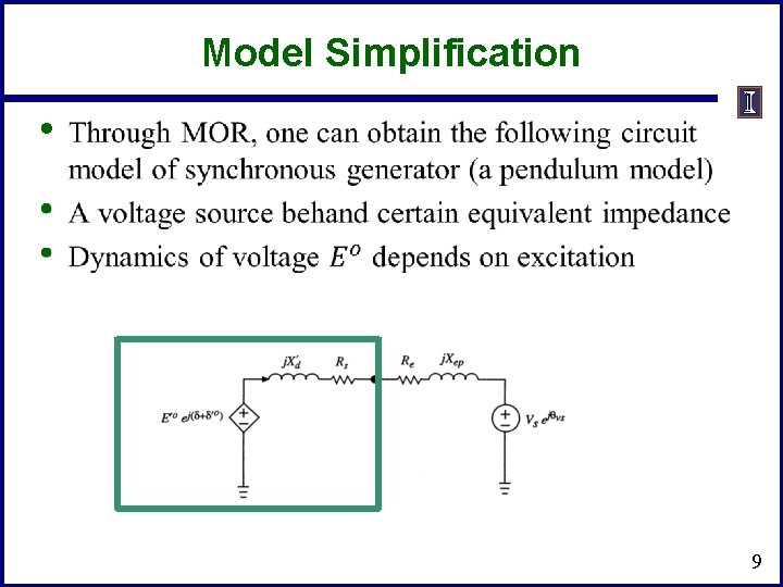
Model Simplification • 9

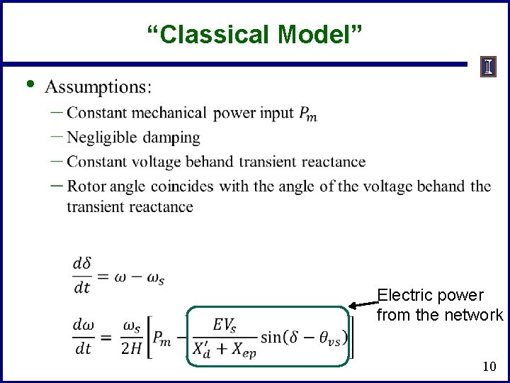
“Classical Model” • Electric power from the network 10

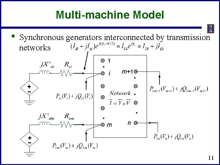
Multi-machine Model • Synchronous generators interconnected by transmission networks 1 i m+1 m n + - 11

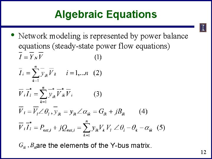
Algebraic Equations • Network modeling is represented by power balance equations (steady-state power flow equations) are the elements of the Y-bus matrix. 12

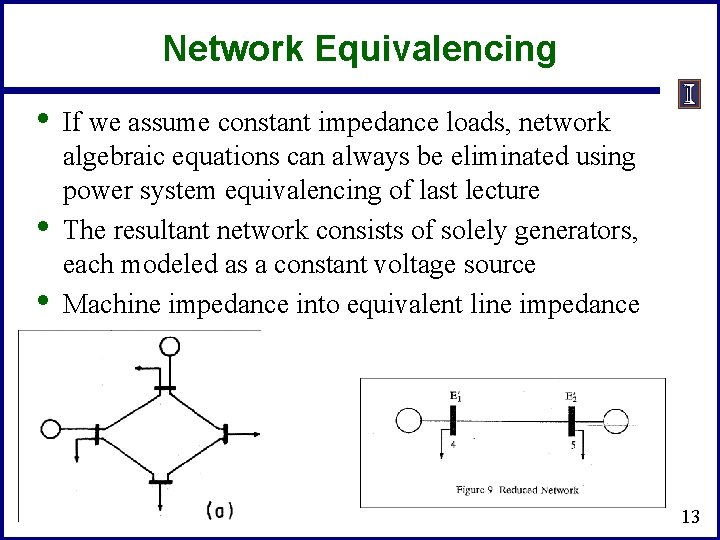
Network Equivalencing • • • If we assume constant impedance loads, network algebraic equations can always be eliminated using power system equivalencing of last lecture The resultant network consists of solely generators, each modeled as a constant voltage source Machine impedance into equivalent line impedance 13

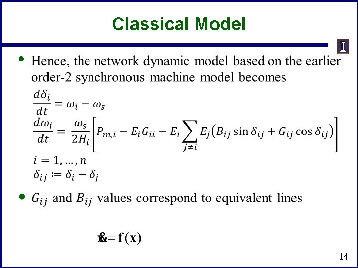
Classical Model • 14

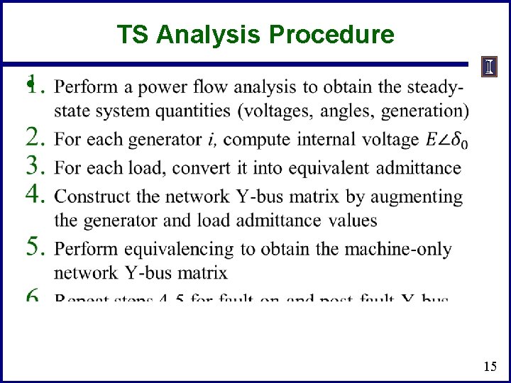
TS Analysis Procedure • 15

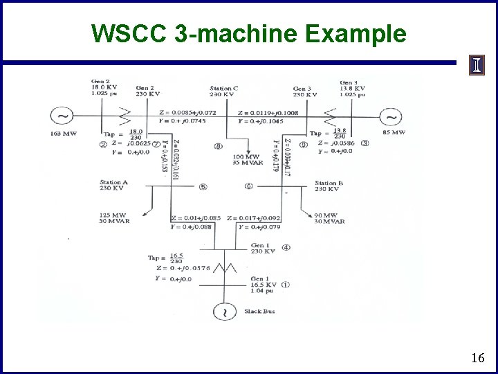
WSCC 3 -machine Example 16

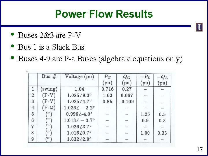
Power Flow Results • • • Buses 2&3 are P-V Bus 1 is a Slack Buses 4 -9 are P-a Buses (algebraic equations only) 17

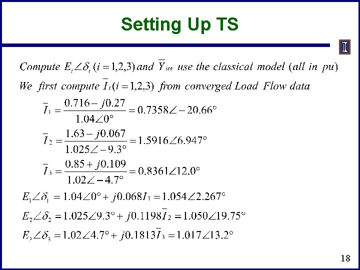
Setting Up TS 18

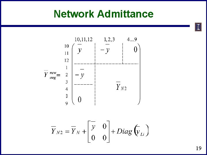
Network Admittance 19

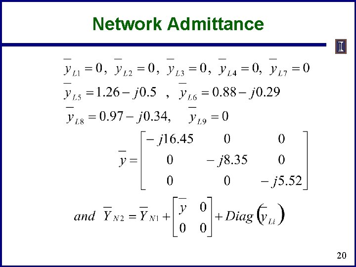
Network Admittance 20

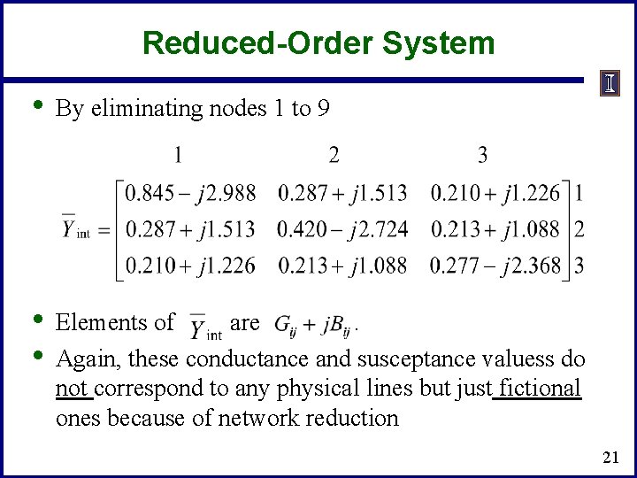
Reduced-Order System • By eliminating nodes 1 to 9 • • Elements of are . Again, these conductance and susceptance valuess do not correspond to any physical lines but just fictional ones because of network reduction 21

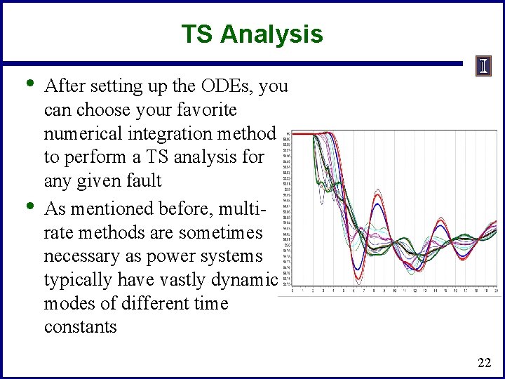
TS Analysis • • After setting up the ODEs, you can choose your favorite numerical integration method to perform a TS analysis for any given fault As mentioned before, multirate methods are sometimes necessary as power systems typically have vastly dynamic modes of different time constants 22

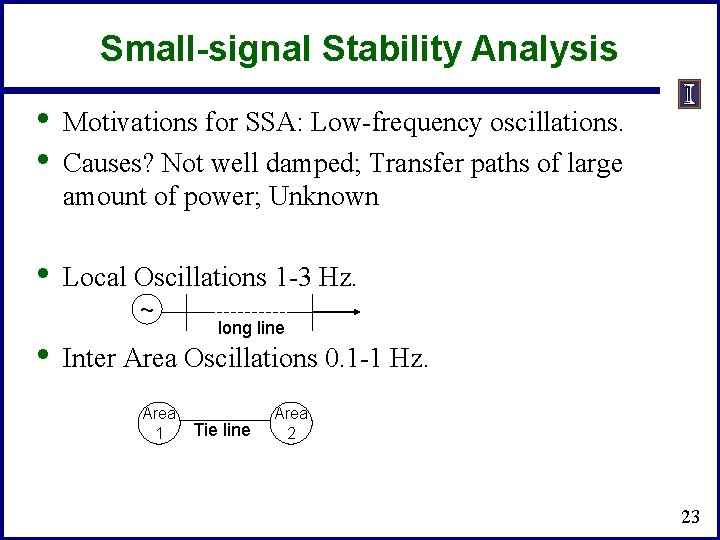
Small-signal Stability Analysis • • Motivations for SSA: Low-frequency oscillations. Causes? Not well damped; Transfer paths of large amount of power; Unknown • Local Oscillations 1 -3 Hz. ~ • long line Inter Area Oscillations 0. 1 -1 Hz. Area 1 Tie line Area 2 23

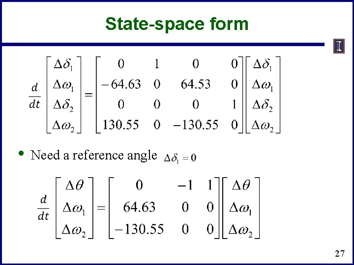
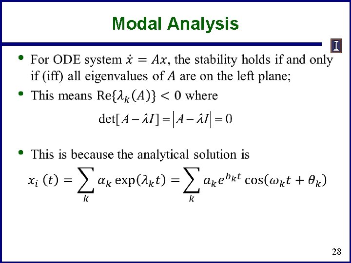
Techniques for SSA • Both DAE and ODE models can be used. • Industry favors a numerical approach using DAE. • In DAE models, after linearizing, the algebraic equations are eliminated to compute eigenvalues. • Eigenvalues, eigenvectors of the linearized system give lots of insight on SSA. 24

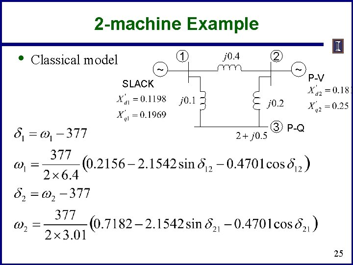
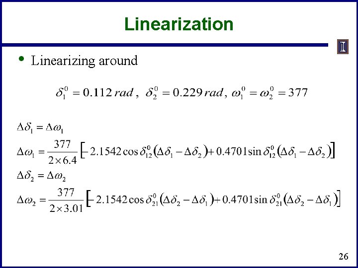
2 -machine Example • 1 Classical model ~ 2 ~ SLACK P-V 3 P-Q 25

Linearization • Linearizing around 26

State-space form • Need a reference angle 27

Modal Analysis • 28

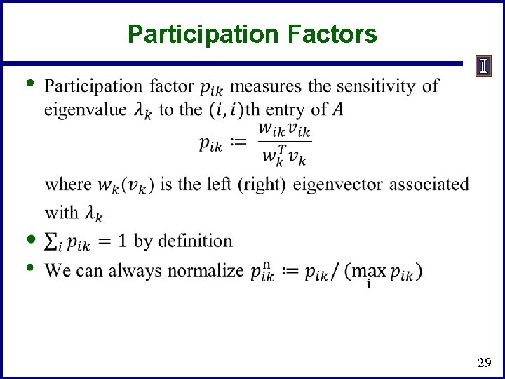
Participation Factors • 29

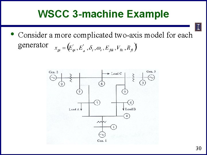
WSCC 3 -machine Example • Consider a more complicated two-axis model for each generator 30

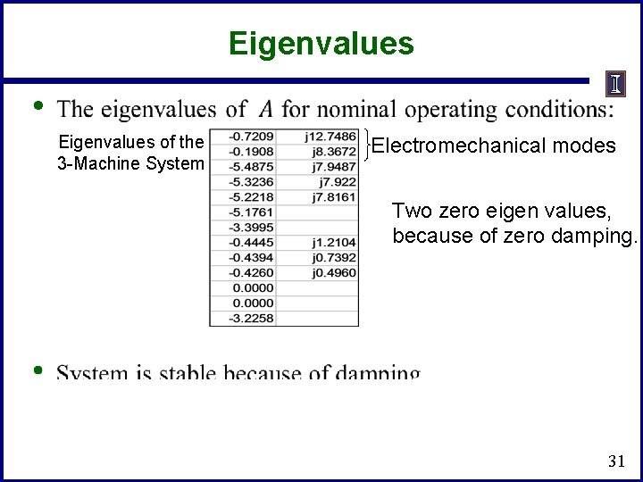
Eigenvalues • Eigenvalues of the 3 -Machine System Electromechanical modes Two zero eigen values, because of zero damping. 31

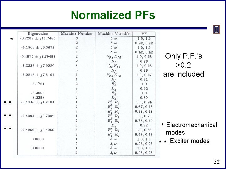
Normalized PFs * Only P. F. ’s >0. 2 are included * * * * Electromechanical modes * * Exciter modes 32