Week 2 1 Week 2 2 oil oil

Week 2. 1

Week 2. 2

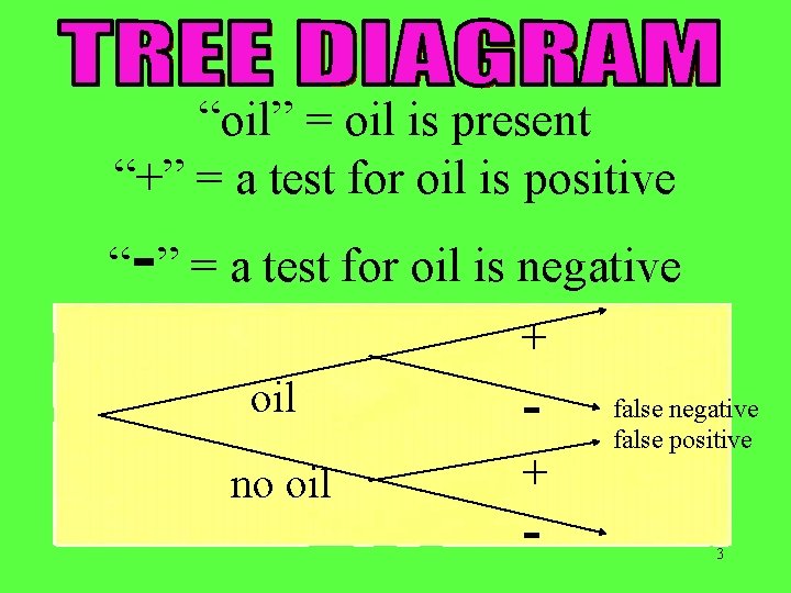
“oil” = oil is present “+” = a test for oil is positive - “ ” = a test for oil is negative + oil - no oil + - false negative false positive 3

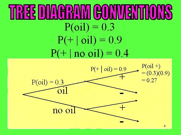
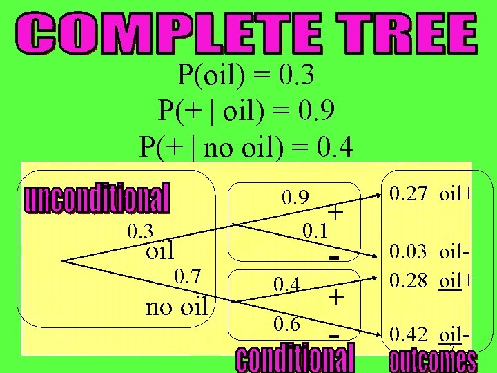
P(oil) = 0. 3 P(+ | oil) = 0. 9 P(+ | no oil) = 0. 4 P(+ | oil) = 0. 9 P(oil) = 0. 3 + oil - no oil + - P(oil +) = (0. 3)(0. 9) = 0. 27 4

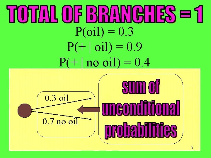
P(oil) = 0. 3 P(+ | oil) = 0. 9 P(+ | no oil) = 0. 4 0. 3 oil 0. 7 no oil 5

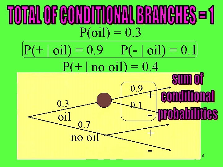
P(oil) = 0. 3 P(+ | oil) = 0. 9 P(- | oil) = 0. 1 P(+ | no oil) = 0. 4 0. 9 0. 3 oil 0. 1 0. 7 no oil + + - 6

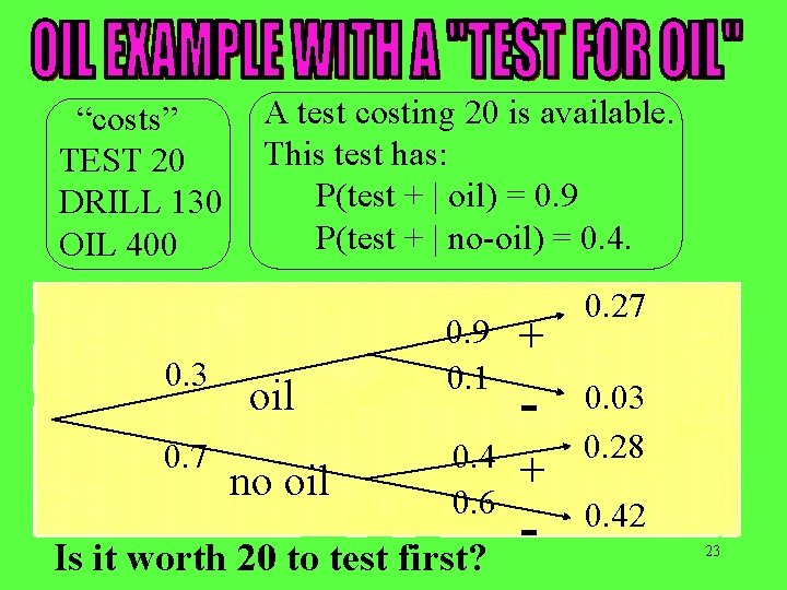
P(oil) = 0. 3 P(+ | oil) = 0. 9 P(+ | no oil) = 0. 4 0. 3 oil 0. 7 no oil 0. 9 + 0. 1 0. 4 0. 6 - + - 0. 27 oil+ 0. 03 oil 0. 28 oil+ 0. 42 oil 7

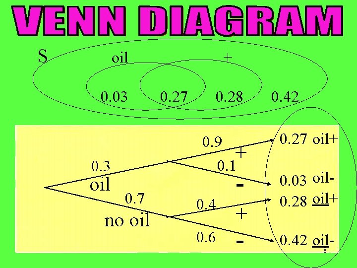
S oil 0. 03 0. 27 0. 28 0. 9 + 0. 1 0. 3 oil + 0. 7 no oil 0. 4 0. 6 - + - 0. 42 0. 27 oil+ 0. 03 oil 0. 28 oil+ 0. 42 oil 8

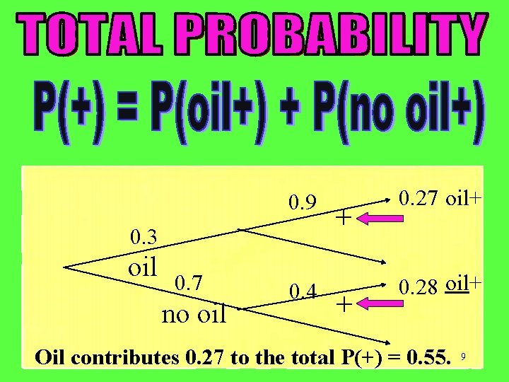
0. 9 0. 3 oil 0. 7 no oil 0. 4 + + 0. 27 oil+ 0. 28 oil+ Oil contributes 0. 27 to the total P(+) = 0. 55. 9

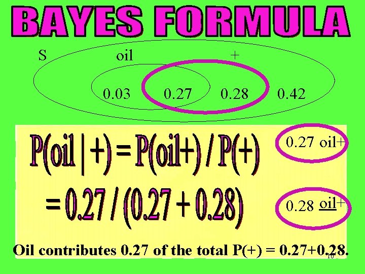
S oil 0. 03 + 0. 27 0. 28 0. 42 0. 27 oil+ 0. 28 oil+ Oil contributes 0. 27 of the total P(+) = 0. 27+0. 28. 10

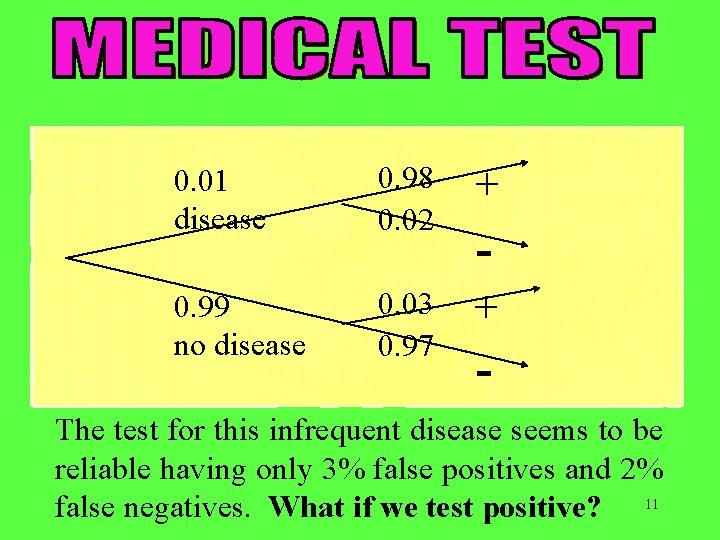
0. 01 disease 0. 98 0. 02 + 0. 99 no disease 0. 03 0. 97 + - The test for this infrequent disease seems to be reliable having only 3% false positives and 2% false negatives. What if we test positive? 11

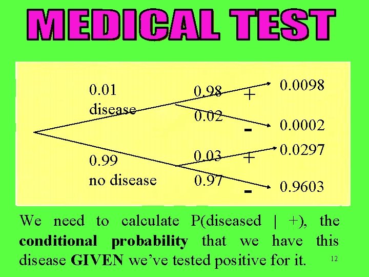
0. 01 disease 0. 98 0. 02 + 0. 0098 - 0. 99 no disease 0. 03 0. 97 + 0. 0002 0. 0297 - 0. 9603 We need to calculate P(diseased | +), the conditional probability that we have this disease GIVEN we’ve tested positive for it. 12

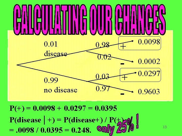
0. 01 disease 0. 98 0. 02 + 0. 0098 - 0. 99 no disease 0. 03 0. 97 + 0. 0002 0. 0297 - P(+) = 0. 0098 + 0. 0297 = 0. 0395 P(disease | +) = P(disease+) / P(+) =. 0098 / 0. 0395 = 0. 248. 0. 9603 13

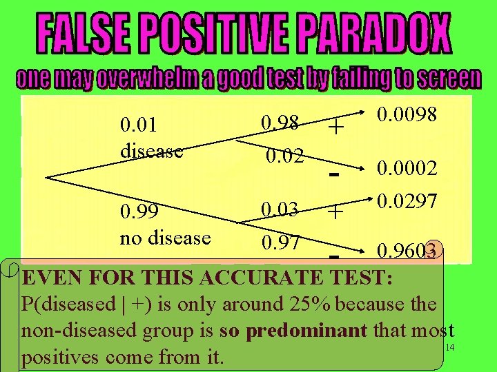
0. 01 disease 0. 98 0. 02 + 0. 0098 - 0. 99 no disease 0. 03 0. 97 + 0. 0002 0. 0297 0. 9603 EVEN FOR THIS ACCURATE TEST: P(diseased | +) is only around 25% because the non-diseased group is so predominant that most 14 positives come from it.

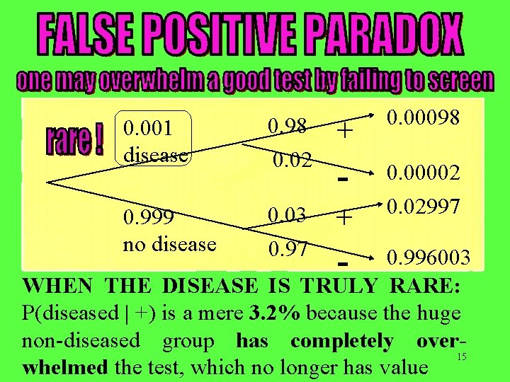
0. 001 disease 0. 98 0. 02 + 0. 00098 - 0. 999 no disease 0. 03 0. 97 + 0. 00002 0. 02997 - 0. 996003 WHEN THE DISEASE IS TRULY RARE: P(diseased | +) is a mere 3. 2% because the huge non-diseased group has completely over 15 whelmed the test, which no longer has value

FOR MEDICAL PRACTICE: Good diagnostic tests will be of little use if the system is overwhelmed by lots of healthy people taking the test. Screen patients first. FOR BUSINESS: Good sales people capably focus their efforts on likely buyers, leading to increased sales. They can be rendered ineffective by feeding them too many false leads, as with massive un-targeted sales promotions. 16

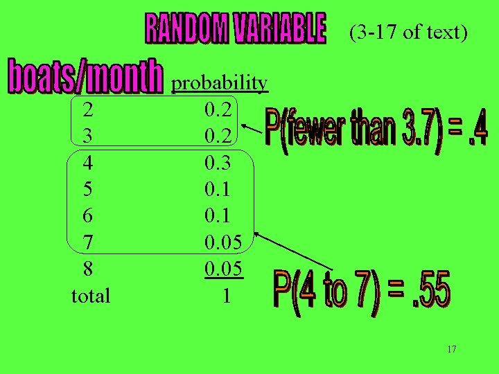
(3 -17 of text) 2 3 4 5 6 7 8 total probability 0. 2 0. 3 0. 1 0. 05 1 17

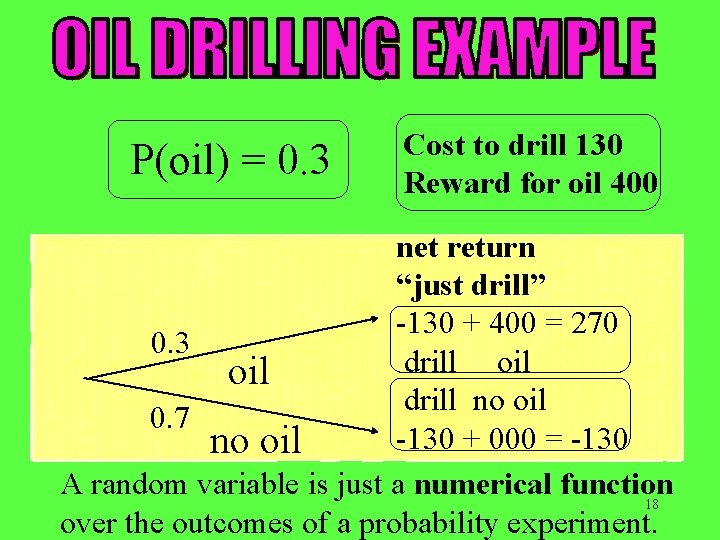
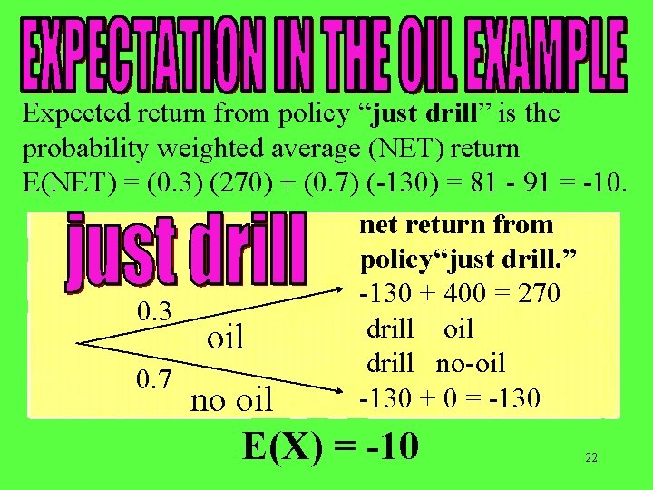
P(oil) = 0. 3 Cost to drill 130 Reward for oil 400 net return “just drill” -130 + 400 = 270 0. 3 drill oil drill no oil 0. 7 -130 + 000 = -130 no oil A random variable is just a numerical function 18 over the outcomes of a probability experiment.

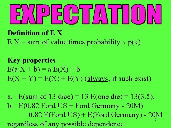
Definition of E X = sum of value times probability x p(x). Key properties E(a X + b) = a E(X) + b E(X + Y) = E(X) + E(Y) (always, if such exist) a. E(sum of 13 dice) = 13 E(one die) = 13(3. 5). b. E(0. 82 Ford US + Ford Germany - 20 M) = 0. 82 E(Ford US) + E(Ford Germany) - 20 M 19 regardless of any possible dependence.

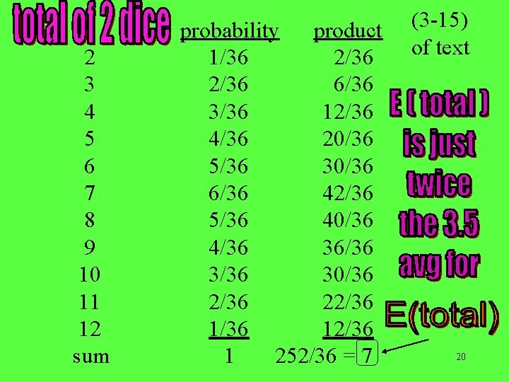
2 3 4 5 6 7 8 9 10 11 12 sum probability product 1/36 2/36 6/36 3/36 12/36 4/36 20/36 5/36 30/36 6/36 42/36 5/36 40/36 4/36 36/36 30/36 22/36 12/36 1 252/36 = 7 (3 -15) of text 20

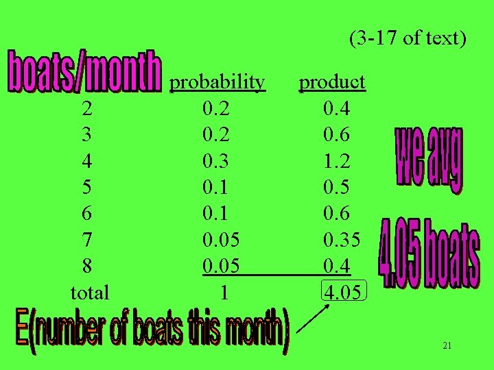
(3 -17 of text) 2 3 4 5 6 7 8 total probability 0. 2 0. 3 0. 1 0. 05 1 product 0. 4 0. 6 1. 2 0. 5 0. 6 0. 35 0. 4 4. 05 21

Expected return from policy “just drill” is the probability weighted average (NET) return E(NET) = (0. 3) (270) + (0. 7) (-130) = 81 - 91 = -10. net return from policy“just drill. ” -130 + 400 = 270 0. 3 drill oil drill no-oil 0. 7 -130 + 0 = -130 no oil E(X) = -10 22

“costs” TEST 20 DRILL 130 OIL 400 0. 3 0. 7 A test costing 20 is available. This test has: P(test + | oil) = 0. 9 P(test + | no-oil) = 0. 4. oil no oil 0. 9 0. 1 + 0. 4 0. 6 + Is it worth 20 to test first? - 0. 27 0. 03 0. 28 0. 42 23

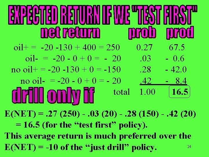
oil+ = -20 -130 + 400 = 250 0. 27 oil- = -20 - 0 + 0 = - 20. 03 no oil+ = -20 -130 + 0 = -150. 28 no oil- = -20 - 0 + 0 = - 20. 42 total 1. 00 67. 5 - 0. 6 - 42. 0 - 8. 4 16. 5 E(NET) =. 27 (250) -. 03 (20) -. 28 (150) -. 42 (20) = 16. 5 (for the “test first” policy). This average return is much preferred over the 24 E(NET) = -10 of the “just drill” policy.

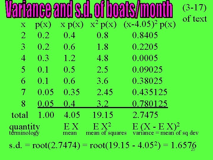
x p(x) 2 0. 2 3 0. 2 4 0. 3 5 0. 1 6 0. 1 7 0. 05 8 0. 05 total 1. 00 quantity terminology x p(x) x 2 p(x) (x-4. 05)2 p(x) 0. 4 0. 8405 0. 6 1. 8 0. 2205 1. 2 4. 8 0. 0005 0. 5 2. 5 0. 09025 0. 6 3. 6 0. 38025 0. 35 2. 45 0. 435125 0. 4 3. 2 0. 780125 4. 05 19. 15 2. 7475 EX E X 2 E (X - E X)2 mean of squares (3 -17) of text variance = mean of sq dev s. d. = root(2. 7474) = root(19. 15 - 4. 052) = 1. 6576 25

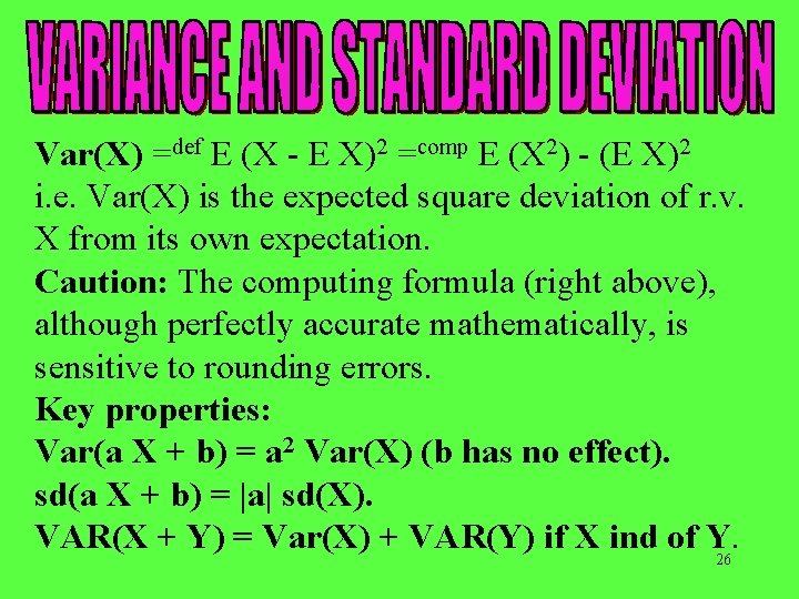
Var(X) =def E (X - E X)2 =comp E (X 2) - (E X)2 i. e. Var(X) is the expected square deviation of r. v. X from its own expectation. Caution: The computing formula (right above), although perfectly accurate mathematically, is sensitive to rounding errors. Key properties: Var(a X + b) = a 2 Var(X) (b has no effect). sd(a X + b) = |a| sd(X). VAR(X + Y) = Var(X) + VAR(Y) if X ind of Y. 26

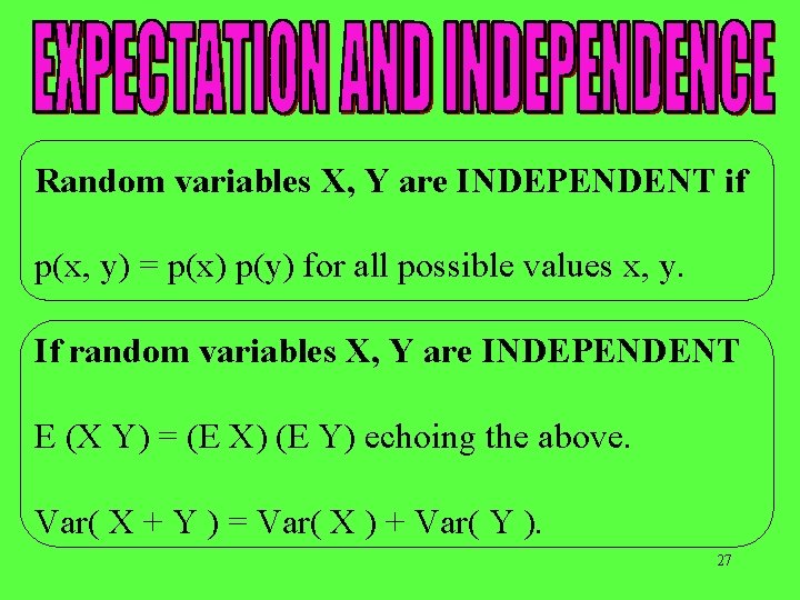
Random variables X, Y are INDEPENDENT if p(x, y) = p(x) p(y) for all possible values x, y. If random variables X, Y are INDEPENDENT E (X Y) = (E X) (E Y) echoing the above. Var( X + Y ) = Var( X ) + Var( Y ). 27

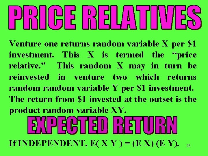
Venture one returns random variable X per $1 investment. This X is termed the “price relative. ” This random X may in turn be reinvested in venture two which returns random variable Y per $1 investment. The return from $1 invested at the outset is the product random variable XY. If INDEPENDENT, E( X Y ) = (E X) (E Y). 28

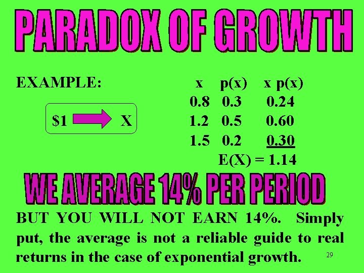
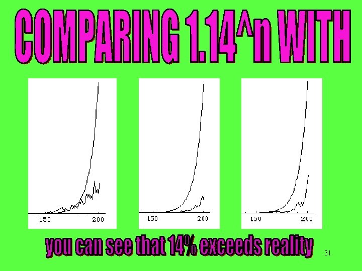
EXAMPLE: $1 X x 0. 8 1. 2 1. 5 p(x) x p(x) 0. 3 0. 24 0. 5 0. 60 0. 2 0. 30 E(X) = 1. 14 BUT YOU WILL NOT EARN 14%. Simply put, the average is not a reliable guide to real returns in the case of exponential growth. 29

EXAMPLE: $1 X x p(x) Log[x] p(x) 0. 8 0. 3 -0. 029073 1. 2 0. 5 0. 039591 1. 5 0. 2 0. 035218 E Log 10[X] = 0. 105311 100. 105311. . = 1. 11106. . With INDEPENDENT plays your RANDOM return will compound at 11. 1% not 14%. (more about this later in the course) 30

31

32