Verification Lisa Holts Kevin Werner Outline Motivation Verification

Verification Lisa Holts Kevin Werner

Outline • Motivation • Verification capabilities • Example

Motivations • Improve understanding of uncertainty from forecast tools – – How good are our forecasts? How much value do human forecasters add? Is one tool better than another? How do the above questions depend on lead time? Amount of runoff? • Can we use what we learn to: – – Improve forecasts? Make forecast process more efficient? Improve collaboration? Convey uncertainty to our users?

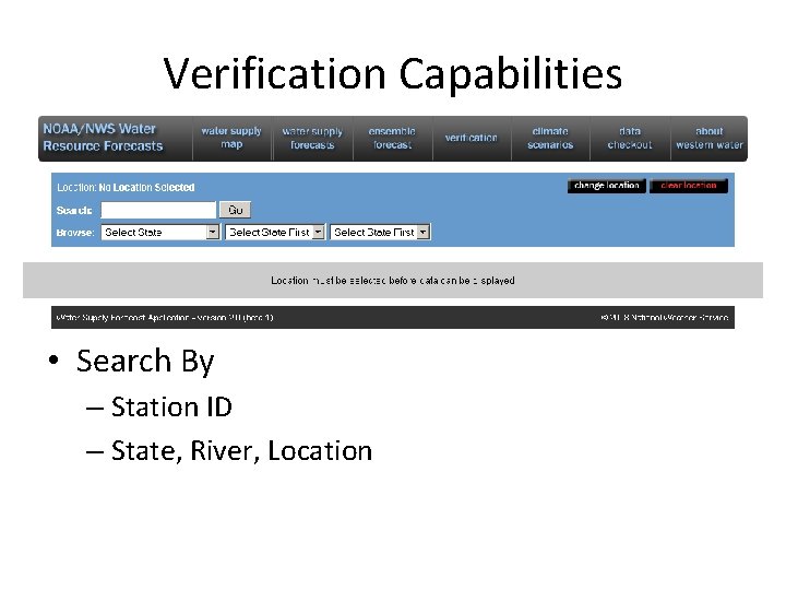
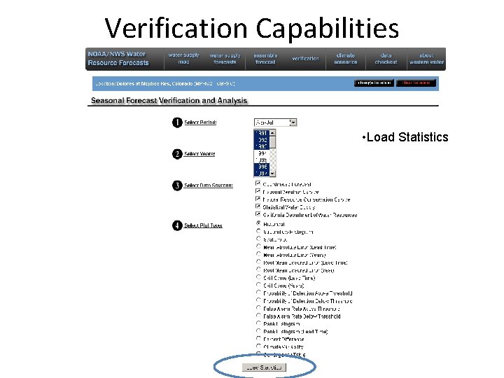
Verification Capabilities • Search By – Station ID – State, River, Location

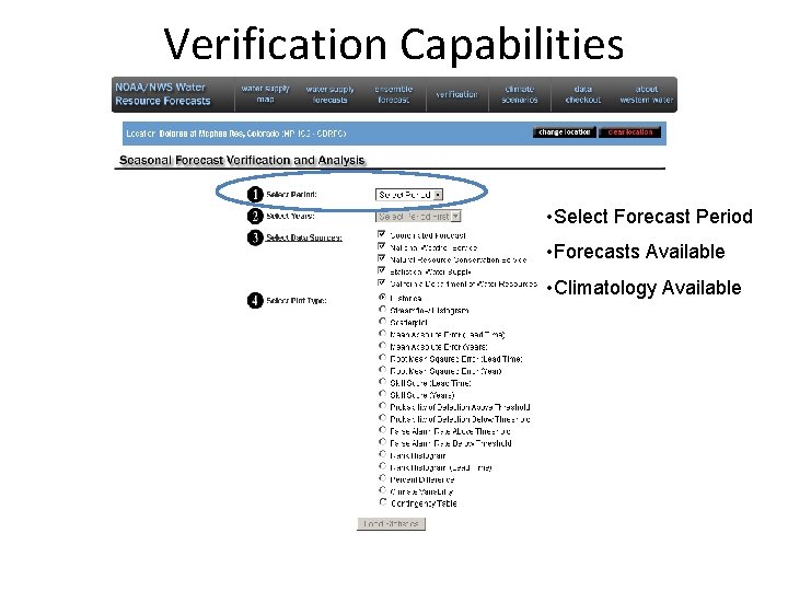
Verification Capabilities • Select Forecast Period • Forecasts Available • Climatology Available

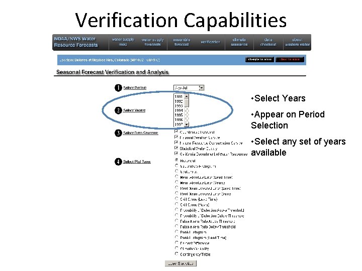
Verification Capabilities • Select Years • Appear on Period Selection • Select any set of years available

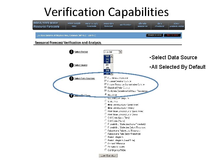
Verification Capabilities • Select Data Source • All Selected By Default

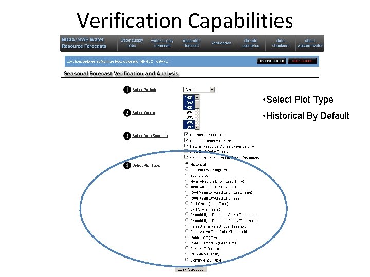
Verification Capabilities • Select Plot Type • Historical By Default

Verification Capabilities • Load Statistics

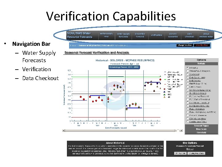
Verification Capabilities • Navigation Bar – Water Supply Forecasts – Verification – Data Checkout

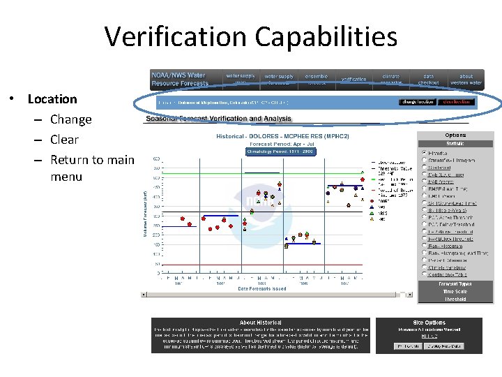
Verification Capabilities • Location – Change – Clear – Return to main menu

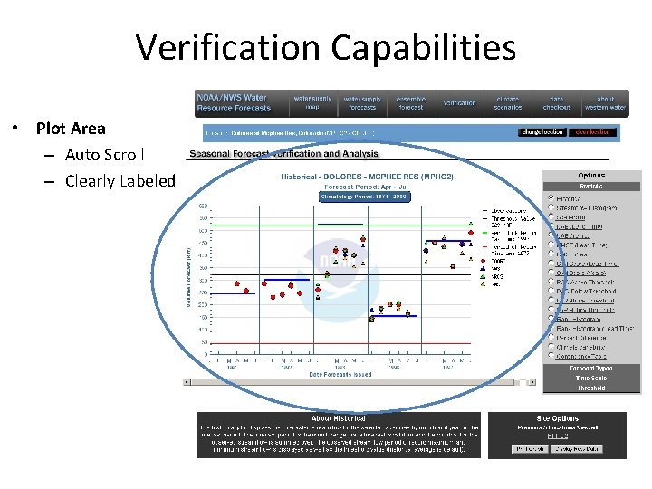
Verification Capabilities • Plot Area – Auto Scroll – Clearly Labeled

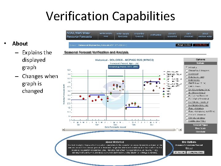
Verification Capabilities • About – Explains the displayed graph – Changes when graph is changed

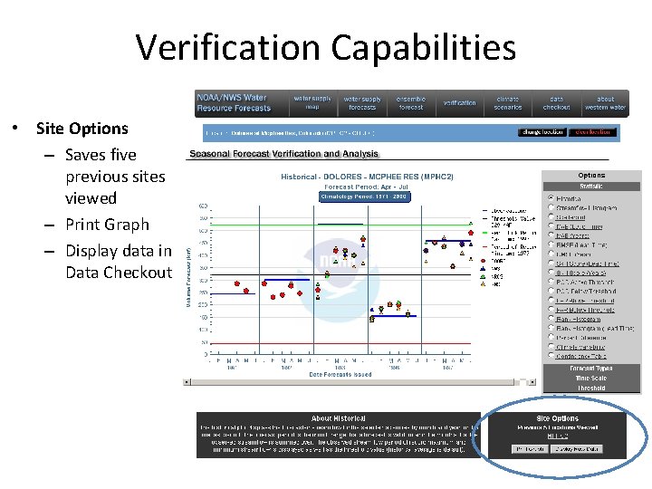
Verification Capabilities • Site Options – Saves five previous sites viewed – Print Graph – Display data in Data Checkout

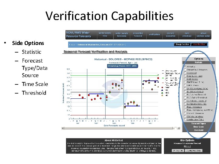
Verification Capabilities • Side Options – Statistic – Forecast Type/Data Source – Time Scale – Threshold

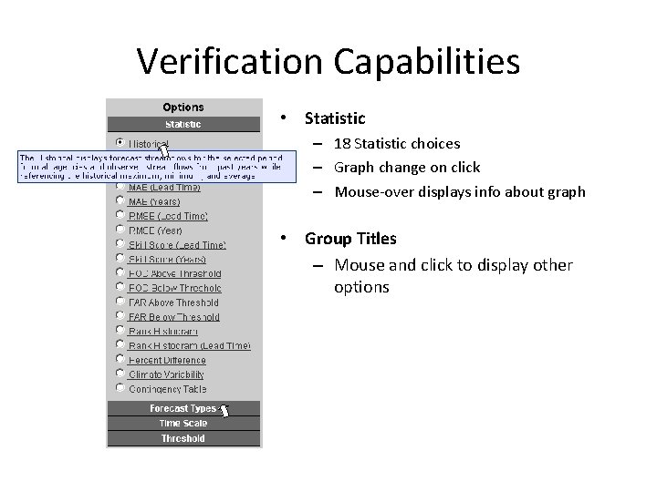
Verification Capabilities • Statistic – 18 Statistic choices – Graph change on click – Mouse-over displays info about graph • Group Titles – Mouse and click to display other options

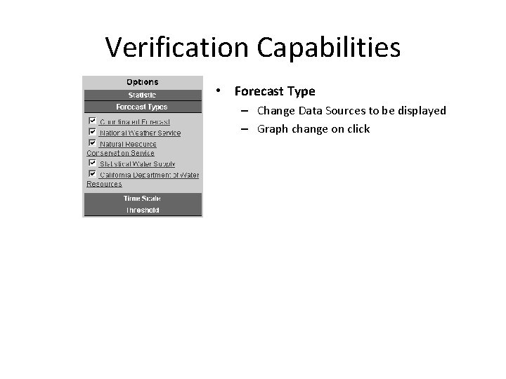
Verification Capabilities • Forecast Type – Change Data Sources to be displayed – Graph change on click

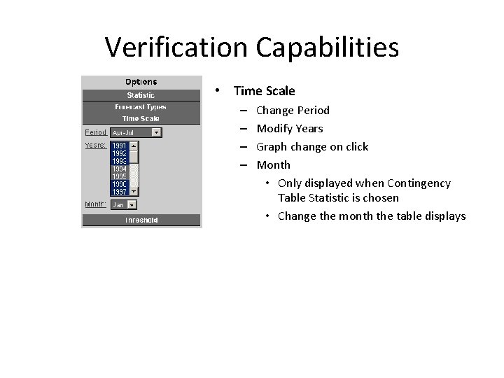
Verification Capabilities • Time Scale – – Change Period Modify Years Graph change on click Month • Only displayed when Contingency Table Statistic is chosen • Change the month the table displays

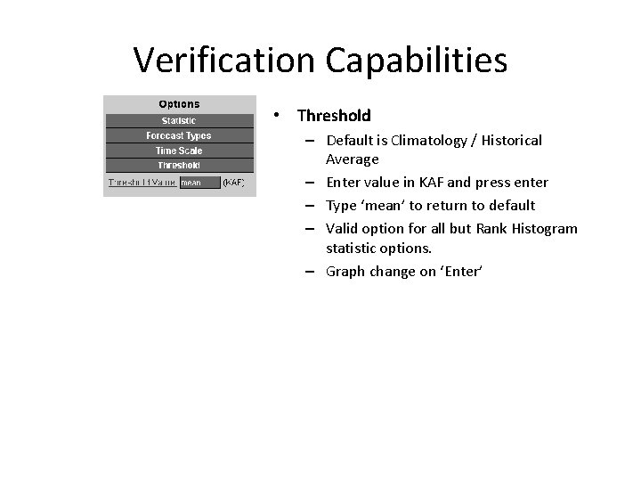
Verification Capabilities • Threshold – Default is Climatology / Historical Average – Enter value in KAF and press enter – Type ‘mean’ to return to default – Valid option for all but Rank Histogram statistic options. – Graph change on ‘Enter’

Assignment • Loose instructions provided • Results should drive study • Goal is not to see five sets of the same plots… rather something focused on the interesting parts for the basin involved

Assignment (con’t) • Step 1: Identify forecast points with extensive data and interest • Step 2: Examine data for visual clues • Step 3: Error and skill scores • Step 4: Categorical statistics • Step 5: Forecast uncertainty • Step 6: Climate variability • Step 7: Snow / Precipitation connections

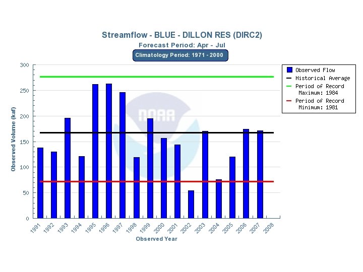
Example • DIRC 2 has forecast / observation pairs from 1991 on. • We’ll look at the available plots and then consolidate it into the case study…

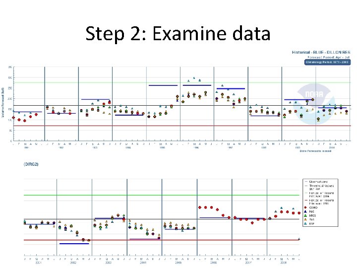
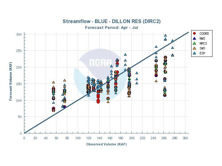
Step 2: Examine data

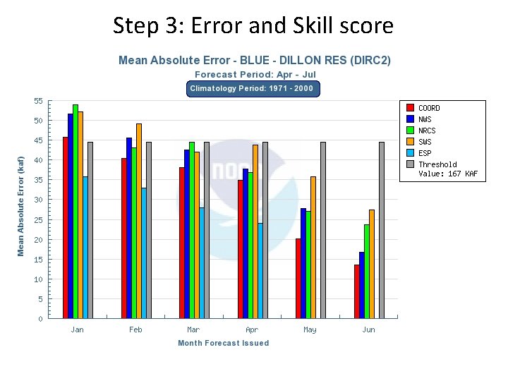
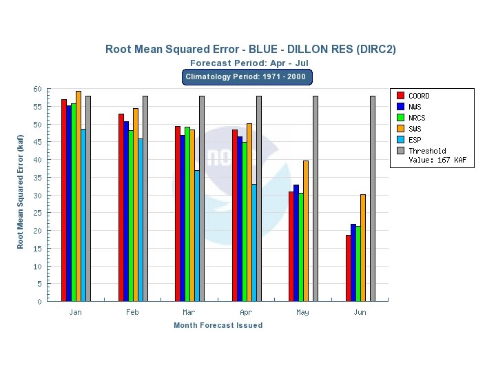
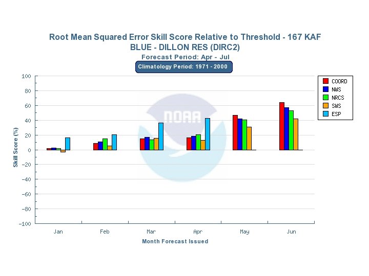
Step 3: Error and Skill score

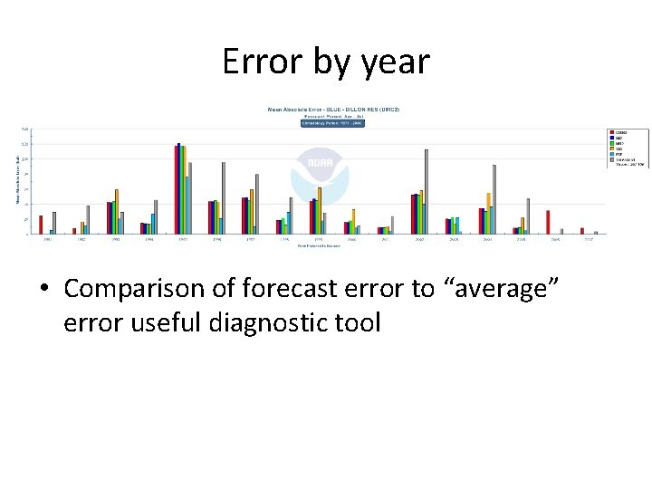
Error by year • Comparison of forecast error to “average” error useful diagnostic tool

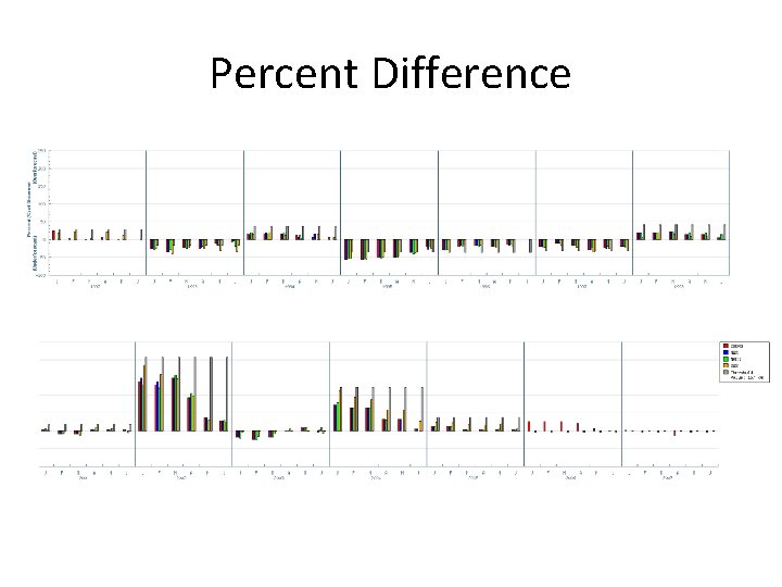
Percent Difference

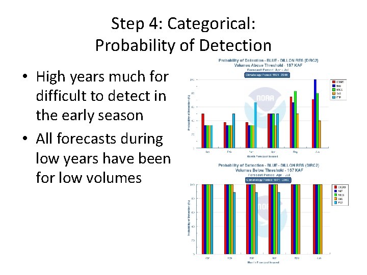
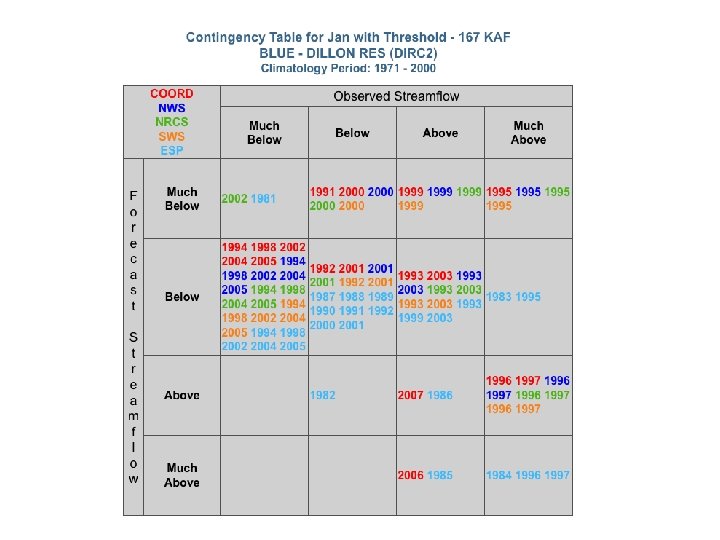
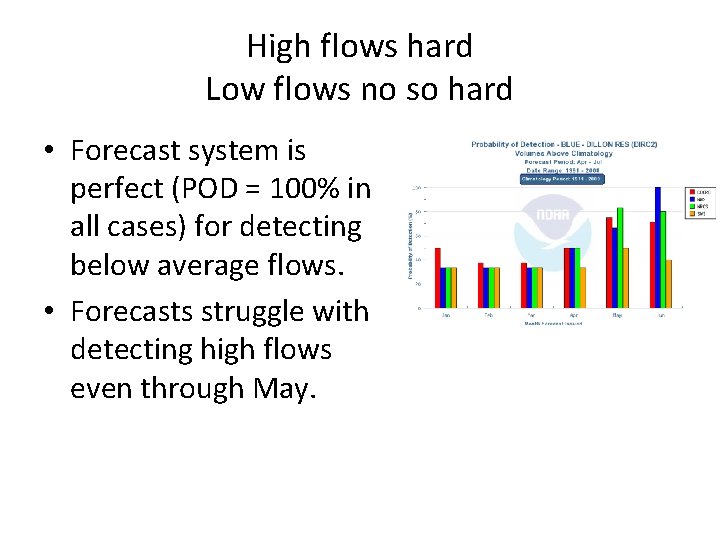
Step 4: Categorical: Probability of Detection • High years much for difficult to detect in the early season • All forecasts during low years have been for low volumes

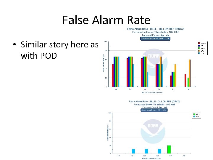
False Alarm Rate • Similar story here as with POD

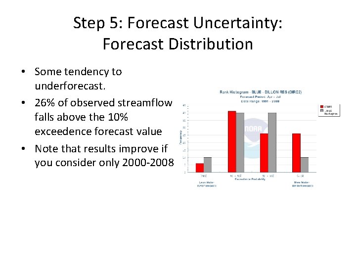
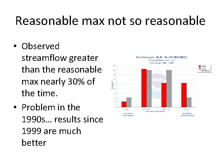
Step 5: Forecast Uncertainty: Forecast Distribution • Some tendency to underforecast. • 26% of observed streamflow falls above the 10% exceedence forecast value • Note that results improve if you consider only 2000 -2008

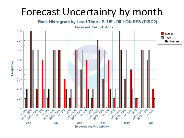
Forecast Uncertainty by month

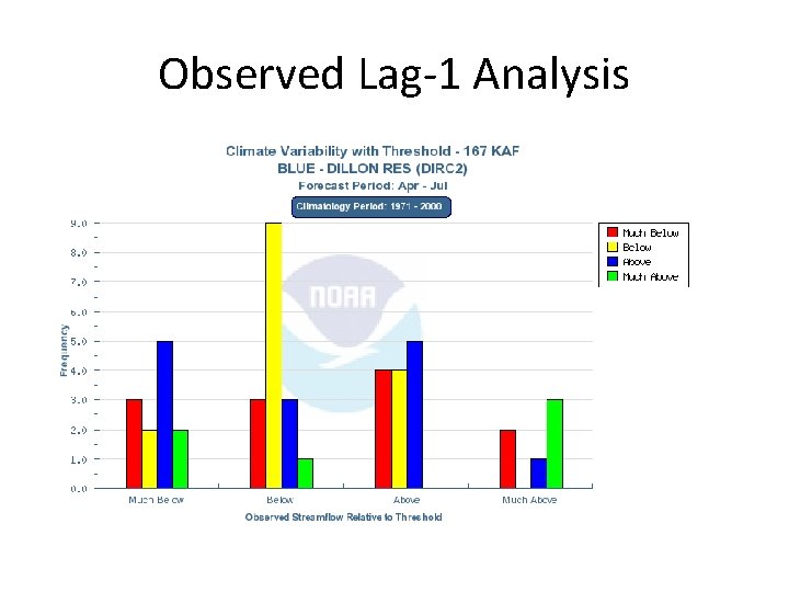
Observed Lag-1 Analysis

Results that might be presented …

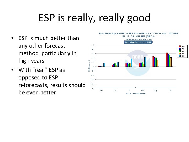
ESP is really, really good • ESP is much better than any other forecast method particularly in high years • With “real” ESP as opposed to ESP reforecasts, results should be even better

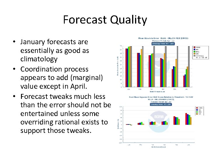
Forecast Quality • January forecasts are essentially as good as climatology • Coordination process appears to add (marginal) value except in April. • Forecast tweaks much less than the error should not be entertained unless some overriding rational exists to support those tweaks.

High flows hard Low flows no so hard • Forecast system is perfect (POD = 100% in all cases) for detecting below average flows. • Forecasts struggle with detecting high flows even through May.

Reasonable max not so reasonable • Observed streamflow greater than the reasonable max nearly 30% of the time. • Problem in the 1990 s… results since 1999 are much better

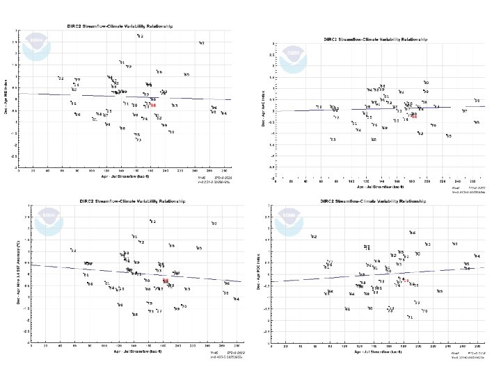
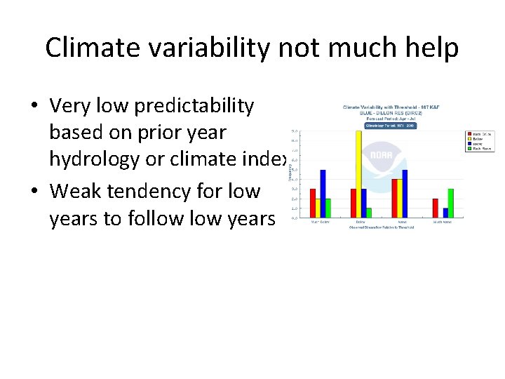
Climate variability not much help • Very low predictability based on prior year hydrology or climate index • Weak tendency for low years to follow years

Possible Application (Discussion) • April DIRC 2 forecast is 150 k. Ac-ft. Average error for April is 35 k. Ac-ft. How could you use this information to: – Improve your forecast? – Improve your forecast process? – Improve forecast application?