UMass Lowell Computer Science 91 503 Analysis of

UMass Lowell Computer Science 91. 503 Analysis of Algorithms Prof. Karen Daniels Fall, 2002 Lecture 1 (Part 3) Tuesday, 9/3/02 Design Patterns for Optimization Problems Dynamic Programming & Greedy Algorithms

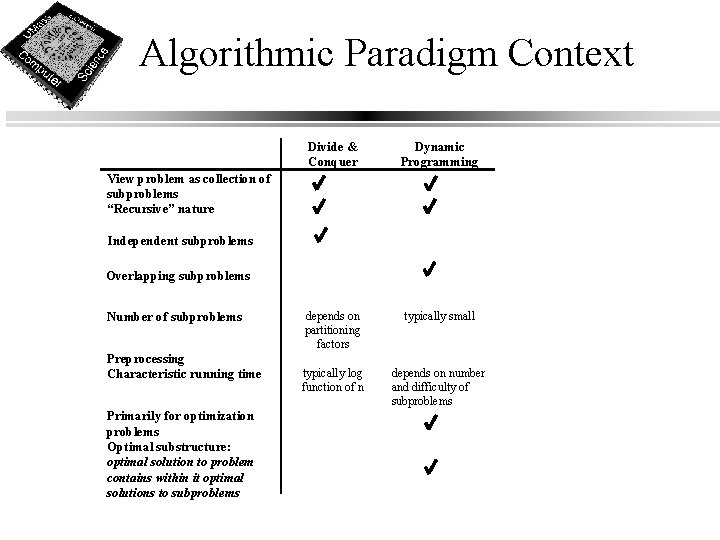
Algorithmic Paradigm Context Divide & Conquer Dynamic Programming depends on partitioning factors typically small typically log function of n depends on number and difficulty of subproblems View problem as collection of subproblems “Recursive” nature Independent subproblems Overlapping subproblems Number of subproblems Preprocessing Characteristic running time Primarily for optimization problems Optimal substructure: optimal solution to problem contains within it optimal solutions to subproblems

Dynamic Programming

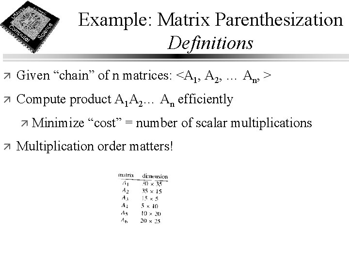
Example: Matrix Parenthesization Definitions ä Given “chain” of n matrices: <A 1, A 2, … An, > ä Compute product A 1 A 2… An efficiently ä Minimize “cost” = number of scalar multiplications ä Multiplication order matters!

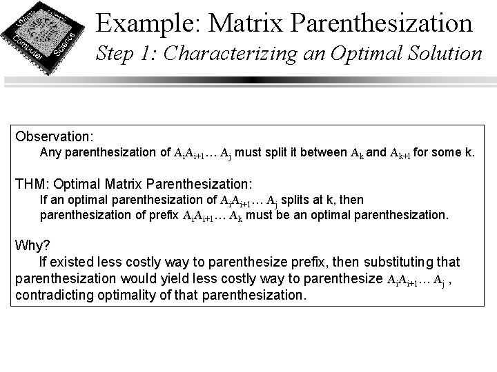
Example: Matrix Parenthesization Step 1: Characterizing an Optimal Solution Observation: Any parenthesization of Ai. Ai+1… Aj must split it between Ak and Ak+1 for some k. THM: Optimal Matrix Parenthesization: If an optimal parenthesization of Ai. Ai+1… Aj splits at k, then parenthesization of prefix Ai. Ai+1… Ak must be an optimal parenthesization. Why? If existed less costly way to parenthesize prefix, then substituting that parenthesization would yield less costly way to parenthesize Ai. Ai+1… Aj , contradicting optimality of that parenthesization.

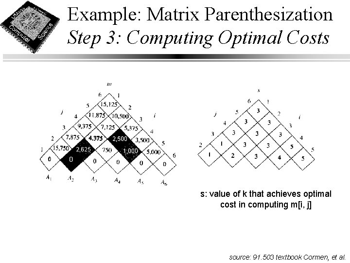
Example: Matrix Parenthesization Step 2: A Recursive Solution ä Recursive definition of minimum parenthesization cost: 0 m[i, j]= min{m[i, k] + m[k+1, j] + pi-1 pkpj} i <= k < j How many distinct subproblems? if i = j if i < j

Example: Matrix Parenthesization Step 3: Computing Optimal Costs 2, 500 2, 625 1, 000 0 s: value of k that achieves optimal cost in computing m[i, j] source: 91. 503 textbook Cormen, et al.

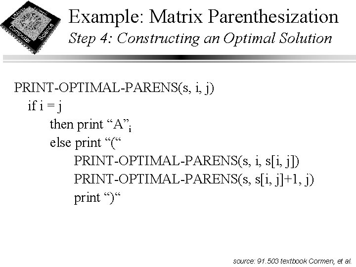
Example: Matrix Parenthesization Step 4: Constructing an Optimal Solution PRINT-OPTIMAL-PARENS(s, i, j) if i = j then print “A”i else print “(“ PRINT-OPTIMAL-PARENS(s, i, s[i, j]) PRINT-OPTIMAL-PARENS(s, s[i, j]+1, j) print “)“ source: 91. 503 textbook Cormen, et al.

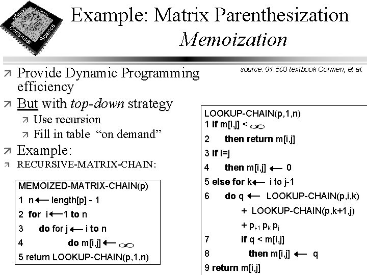
Example: Matrix Parenthesization Memoization ä ä Provide Dynamic Programming efficiency But with top-down strategy ä ä Use recursion Fill in table “on demand” ä Example: ä RECURSIVE-MATRIX-CHAIN: MEMOIZED-MATRIX-CHAIN(p) 1 n length[p] - 1 2 for i 3 4 source: 91. 503 textbook Cormen, et al. LOOKUP-CHAIN(p, 1, n) 1 if m[i, j] < 2 3 if i=j 4 i to n do m[i, j] 5 return LOOKUP-CHAIN(p, 1, n) then m[i, j] 5 else for k 6 do q 0 i to j-1 LOOKUP-CHAIN(p, i, k) + LOOKUP-CHAIN(p, k+1, j) 1 to n do for j then return m[i, j] + pi-1 pk pj 7 8 if q < m[i, j] then m[i, j] 9 return m[i, j] q

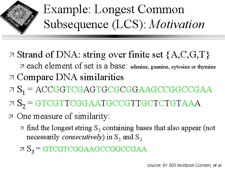
Example: Longest Common Subsequence (LCS): Motivation ä Strand of DNA: string over finite set {A, C, G, T} ä each element of set is a base: adenine, guanine, cytosine or thymine ä Compare DNA similarities ä S 1 = ACCGGTCGAGTGCGCGGAAGCCGAA ä S 2 = GTCGTTCGGAATGCCGTTGCTCTGTAAA ä One measure of similarity: ä find the longest string S 3 containing bases that also appear (not necessarily consecutively) in S 1 and S 2 ä S 3 = GTCGTCGGAAGCCGAA source: 91. 503 textbook Cormen, et al.

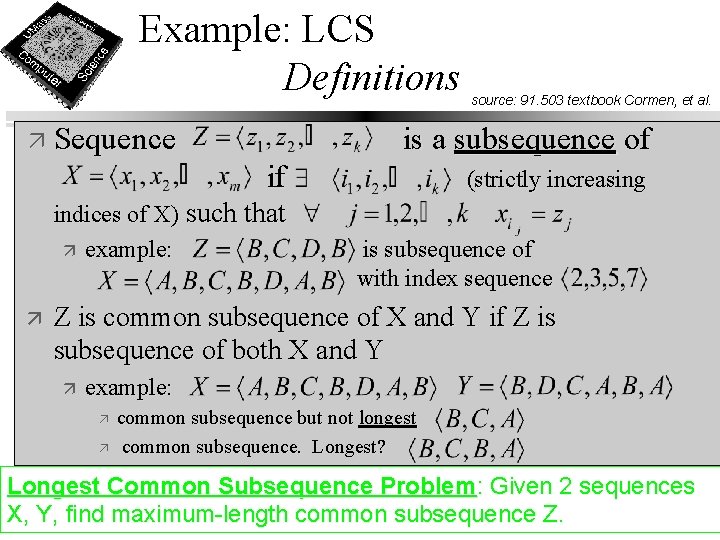
Example: LCS Definitions ä Sequence is a subsequence of if indices of X) such that ä example: ä source: 91. 503 textbook Cormen, et al. (strictly increasing is subsequence of with index sequence Z is common subsequence of X and Y if Z is subsequence of both X and Y ä example: ä ä common subsequence but not longest common subsequence. Longest? Longest Common Subsequence Problem: Given 2 sequences X, Y, find maximum-length common subsequence Z.

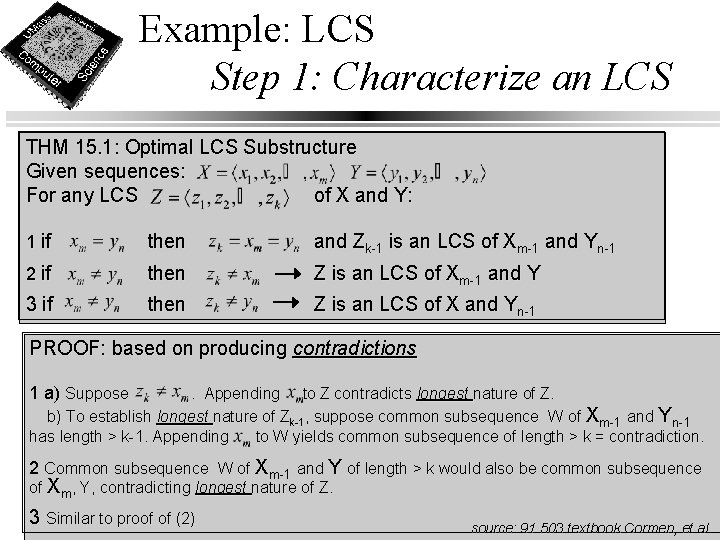
Example: LCS Step 1: Characterize an LCS THM 15. 1: Optimal LCS Substructure Given sequences: For any LCS of X and Y: 1 if then and Zk-1 is an LCS of Xm-1 and Yn-1 2 if then Z is an LCS of Xm-1 and Y 3 if then Z is an LCS of X and Yn-1 PROOF: based on producing contradictions 1 a) Suppose . Appending to Z contradicts longest nature of Z. b) To establish longest nature of Zk-1, suppose common subsequence W of Xm-1 and Yn-1 has length > k-1. Appending to W yields common subsequence of length > k = contradiction. 2 Common subsequence W of Xm-1 and Y of length > k would also be common subsequence of Xm, Y, contradicting longest nature of Z. 3 Similar to proof of (2) source: 91. 503 textbook Cormen, et al.

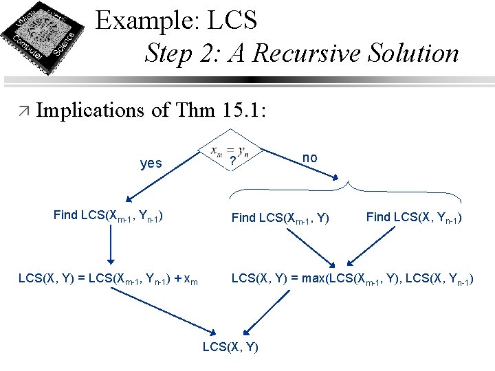
Example: LCS Step 2: A Recursive Solution ä Implications of Thm 15. 1: yes Find LCS(Xm-1, Yn-1) LCS(X, Y) = LCS(Xm-1, Yn-1) + xm ? no Find LCS(Xm-1, Y) Find LCS(X, Yn-1) LCS(X, Y) = max(LCS(Xm-1, Y), LCS(X, Yn-1) LCS(X, Y)

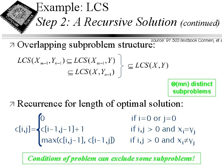
Example: LCS Step 2: A Recursive Solution (continued) source: 91. 503 textbook Cormen, et a ä Overlapping subproblem structure: Q(mn) distinct subproblems ä Recurrence for length of optimal solution: 0 c[i, j]= c[i-1, j-1]+1 max(c[i, j-1], c[i-1, j]) if i=0 or j=0 if i, j > 0 and xi=yj Conditions of problem can exclude some subproblems!

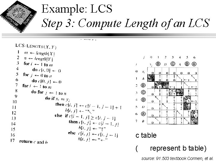
Example: LCS Step 3: Compute Length of an LCS B C B A c table ( represent b table) source: 91. 503 textbook Cormen, et al.

Example: LCS Step 4: Construct an LCS source: 91. 503 textbook Cormen, et al.

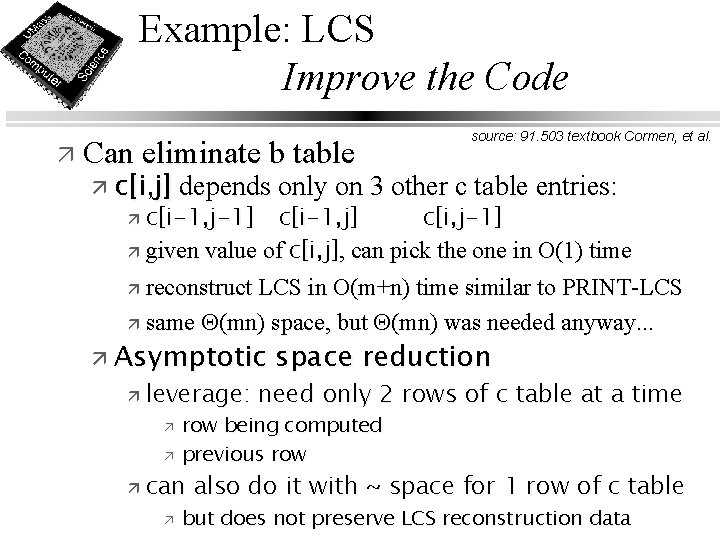
Example: LCS Improve the Code ä Can eliminate b table source: 91. 503 textbook Cormen, et al. ä c[i, j] depends only on 3 other c table entries: c[i-1, j-1] c[i-1, j] c[i, j-1] ä given value of c[i, j], can pick the one in O(1) time ä reconstruct LCS in O(m+n) time similar to PRINT-LCS ä same Q(mn) space, but Q(mn) was needed anyway. . . ä ä Asymptotic ä leverage: need only 2 rows of c table at a time ä ä ä space reduction row being computed previous row can also do it with ~ space for 1 row of c table ä but does not preserve LCS reconstruction data

Algorithmic Paradigm Context

Greedy Algorithms

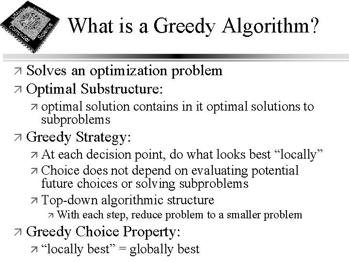
What is a Greedy Algorithm? ä Solves an optimization problem ä Optimal Substructure: ä optimal solution contains in it optimal solutions to subproblems ä Greedy Strategy: ä At each decision point, do what looks best “locally” ä Choice does not depend on evaluating potential future choices or solving subproblems ä Top-down algorithmic structure ä With each step, reduce problem to a smaller problem ä Greedy Choice Property: ä “locally best” = globally best

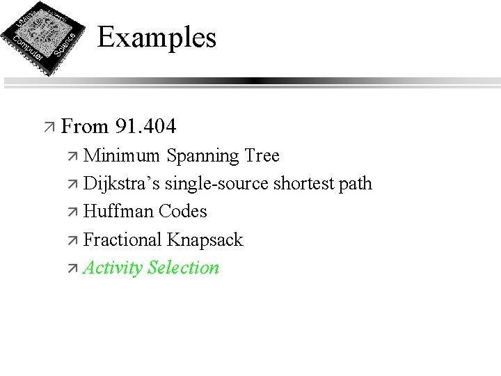
Examples ä From 91. 404 ä Minimum Spanning Tree ä Dijkstra’s single-source shortest path ä Huffman Codes ä Fractional Knapsack ä Activity Selection

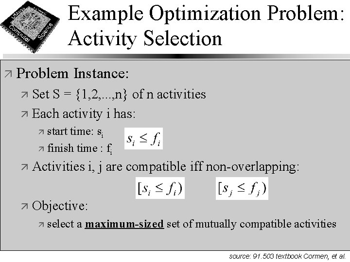
Example Optimization Problem: Activity Selection ä Problem Instance: ä Set S = {1, 2, . . . , n} of n activities ä Each activity i has: start time: si ä finish time : fi ä ä Activities i, j are compatible iff non-overlapping: ä Objective: ä select a maximum-sized set of mutually compatible activities source: 91. 503 textbook Cormen, et al.

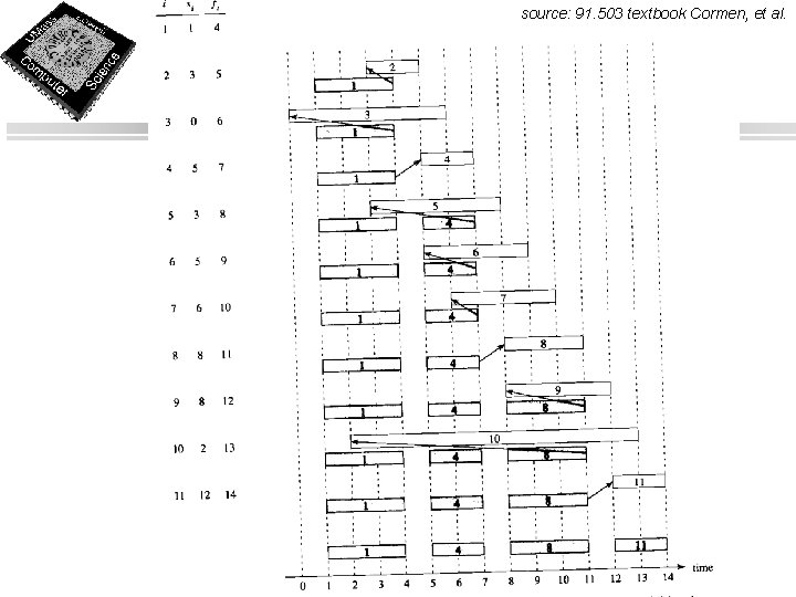
source: 91. 503 textbook Cormen, et al.

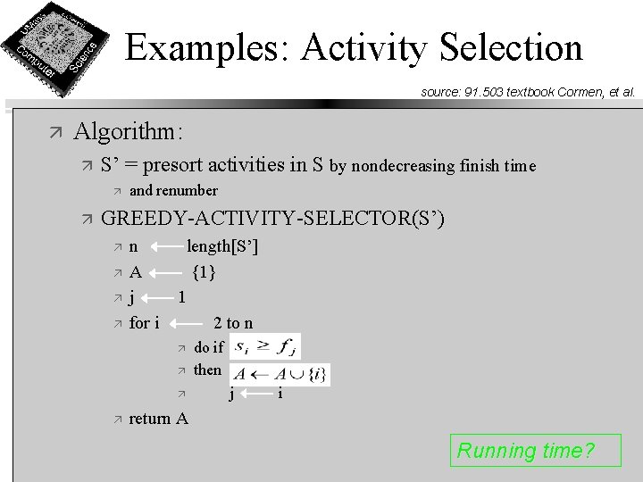
Examples: Activity Selection source: 91. 503 textbook Cormen, et al. ä Algorithm: ä S’ = presort activities in S by nondecreasing finish time ä ä and renumber GREEDY-ACTIVITY-SELECTOR(S’) ä ä n length[S’] A {1} j 1 for i 2 to n ä ä do if then j i return A Running time?

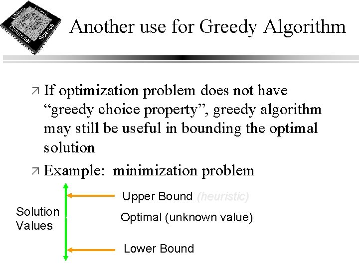
Another use for Greedy Algorithm ä If optimization problem does not have “greedy choice property”, greedy algorithm may still be useful in bounding the optimal solution ä Example: minimization problem Upper Bound (heuristic) Solution Values Optimal (unknown value) Lower Bound