The Variety of Subdivision Schemes Kwan Pyo Ko

The Variety of Subdivision Schemes Kwan Pyo Ko Department of Internet Engineering Dongseo Univ. kpko@dongseo. ac. kr

What is Subdivision? • Define a smooth curves/surface as the limit of a sequence of successive refinements pj + 1 = Spj (Sp) a = X b ®a¡ 2 bpb

Subdivision Surfaces

Why Subdivision? • Arbitrary topology • Multiresolution • Simple code • Efficient code • Construct Wavelet

Chaikin’s Algorithm : = 3 k 1 k p + pi + 1 4 i 4 pk 2 i++11 = 1 k 3 k pi + 1 4 4 pk 2 i+ 1 converges to the quadratic B-spline.

Cubic spline Algorithm : pk 2 i+ 1 = pk 2 i++11 = 1 k p + pi + 1 2 i 2 1 k 3 k 1 pi + 1 + pki+ 2 8 4 8 converges to the cubic B-spline.
: pk 2 i+")
4 -point interpolatory scheme (N. Dyn, D. Levin and J. Gregory): pk 2 i+ 1 = pki µ k+ 1 = p 2 i +1 ¶ 1 + w (pki + pki+ 1 ) ¡ w(pki¡ 2 -continuous for jwj < -C 1 for 0 < w < 18 1 4 1 + pki+ 2 )

Butterfly scheme : X 1 k k k qe = (pe; 1 + pe; 2 ) + 2 w(pe; 3 + pe; 4 ) ¡ w pe; j 2 = 8 j pki + 1 = pki [ qek 5

The mask of the butterfly scheme:

The mask of the butterfly scheme:

Ternary Subdivision Scheme:

pj 3 j+ 1 = pij pj 3 j++11 = apji ¡ i + cpi i + + bp dp j j+1 j+2 1 pj 3 j++12 = dpji ¡ i + bpi i + + cp ap j j+1 j+2 1 where the weights are given by a= ¡ C 2 for 1 1 13 1 7 1 1 1 ¡ w; b = + w; c = ¡ w; d = ¡ + w: 18 6 18 2 18 6 1 15 < w< 1 9

Subdivision Zoo Classification : • stationary or non-stationary • binary or ternary • type of mesh(triangle or quadrilateral) • approximating or interpolating • linear or non-linear
 Triangular meshes 2) approximating Loop (C interpolating Butterfly (C 1)")
Face split (primal type) Triangular meshes 2) approximating Loop (C interpolating Butterfly (C 1) Quad. meshes Catmull-Clark(C Kobbelt (C 2) 1) Vertex split (dual type) Quad. meshes approximating 1 1 Doo-Sabin (C ) , Midedge (C )
 Sr (u) = X")
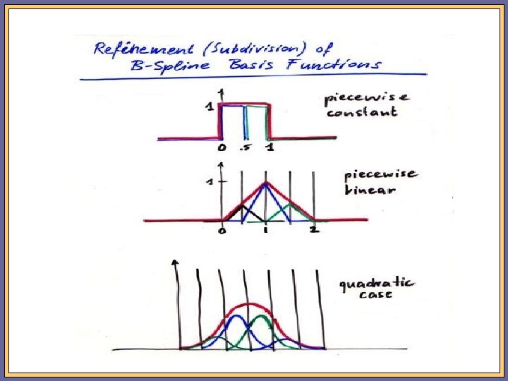
Binary Subdivision of B-splines • Univariate B-splines : ( ¤) Sr (u) = X dri N r (u ¡ i ); i 2 Z where N r : normalized B-spline of degree r:
 = 1")
Properties : P • • • N r (u ¡ i ) = 1 Partition of unity : i r Positivity : N (u) ¸ 0 r Local support : N (u ¡ i ) = 0 if u 2= [i ; i + r + 1] Continuity : N r (u) 2 C ( r ¡ 1) Recursion : N r (u ¡ i ) = u ¡r i N r ¡ 1 (u ¡ i ) + i + r +r 1¡ u N r ¡ 1 (u ¡ i ¡ 1)
 as a curve over")
The idea behind a Subdivision • Rewrite the curve (*) as a curve over a refined knot sequence Z=2: • (*) becomes Sr (u) = X d^rj N r (2(u ¡ j )) j 2 Z =2 • Determine d^jr A single B-spline can be decomposed into similar Bspline of half the support.
 = crj N r (2(u ¡")
• This results in Nr X (u) = crj N r (2(u ¡ j )); j 2 Z =2 crj where = 2¡ d^rj = ¡ r r+1 2 j X ¢ crj ¡ i dri ; j 2 Z=2 i 2 Z • For example. X r = 2 d^20 = c¡ 2 i d 2 i = ¢¢¢+ (3=4)d¡ 2 1 + (1=4)d 20 + ¢¢¢ i 2 Z d^21=2 = ¢¢¢+ (1=4)d¡ 2 1 + (3=4)d 20 + ¢¢¢ Chaikin’s algorithm
 = X dri ; s N")
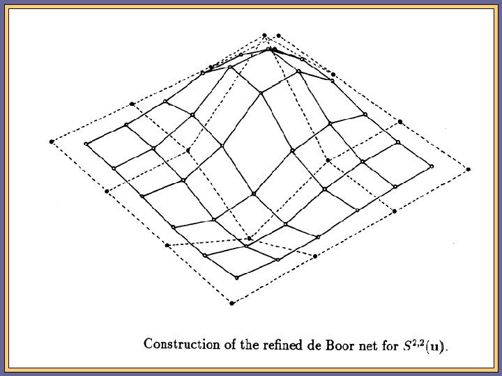
Tensor Product B-spline Surfaces Sr ; s (u) = X dri ; s N r ; s (u ¡ i) i 2 Z 2 A tensor product Bspline is the product of two independently univariate B-splines, i. e N r ; s (u ¡ i) = N r (u ¡ i )N s (v ¡ j )

d^rj ; s = X r ; s 2 crj ; s d ¡ i i ; j 2 Z =2 i 2 Z 2 crj ; s • • = cri csj = 2¡ ( r + s) µ ¶µ ¶ r + 1 s+ 1 2 i 2 j r = s= 2 9 3 ¢¢¢+ ( )d¡ 2; 21; ¡ 1 + ( ) + d 2; 2 ¢¢¢ 0; ¡ 1 + 16 16 3 1 ¢¢¢+ ( )d¡ 2; 21; 0 + ( ) + d 2; 2 ¢¢¢ 0; 0 + 16 16 The mask set : Example 1 = d^2; 2 0; 0

• Example 2 r = s= 3 The mask for bicubic tensor product B-splines
 Sr ; s; t")
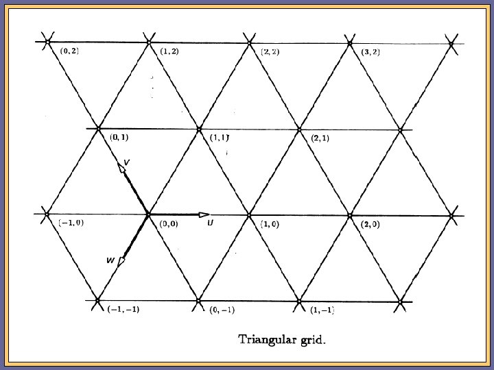
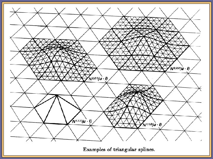
Triangular Splines • A triangular spline surface : ( ¤) Sr ; s; t (u) = X dri ; s; t N r ; s; t (u ¡ i); u 2 R 2; i 2 Z 2 i where N r ; s; t (u) : a normalized triangular spline of degree (r+s+t-2)
 can be rewritten over the refine")
Subdivision of Triangular Splines • The surface (*) can be rewritten over the refine grid. Sr ; s; t (u) = X d^jr ; s; t N r ; s; t 2(u ¡ j ) j • A single triangular spline is decomposed into splines of identical degree over the refined grid. N r ; s; t (u) = X j 2 Z =2 crj ; s; t N r ; s; t (2(u ¡ j ));

d^rj ; s; t = X crj ¡; s; ti dri ; s; t i 2 Z Where crj ; s; t = 2¡ ( r + s+ t ) Xt µ k= 0 r 2 i ¡ k ¶µ ¶µ ¶ s t k 2 j ¡ k 2; 2; 2 (u) The subdivision masks for the triangular spline N
 Subdivision for tensor product quadratic B-spline surface has rigid restrictions")
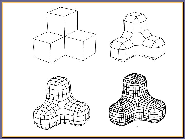
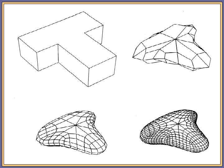
The Doo/Sabin algorithm (Problem) Subdivision for tensor product quadratic B-spline surface has rigid restrictions on the topology. Each vertex of the net must order 4. This restriction makes the design of many surfaces difficult Doo/Sabin presented an algorithm that eliminated this restriction by generalizing the bi-quadratic B-spline subdivision rules to include arbitrary topologies.

P’ 3 P 0 P’’ 0 P 3 P’’ 3 (P 0 ; P 1 ; P 2 ; P 3 ) T = S 4 D S (P 0 ; P 1 ; P 2 ; P 3 ) T P’ 0 P’ 2 P’b 2 P’’ 1 P’’ 2 P’ 1 Doo-Sabin scheme S 4 D S P 2 9 1 6 6 3 = 16 4 1 3 3 9 3 1 1 3 9 3 3 3 1 7 7 3 5 9

• The subdivision masks for bi-quadratic B-spline : • Geometric view of bi-quadratic B-spline subdivision : the new points are centroids of the sub-face formed by the face centroid, a corner vertex and the two midedge points next to the corner. arbitrary topology

• For an n-sided face Doo/Sabin used subdivision matrix Sn. D S = (®i j ) n £ n ; ®i j = = 5+ n 4 n i= j ³ 3 + 2 cos 2¼(ni ¡ 4 n j) ´ 6 j i= • As subdivision proceeds, the refined control point mesh becomes locally rectangular everywhere except at a fixed number of points. • Since bi-quadratic B-splines are C 1 , the surfaces generated by the Doo/Sabin algorithm are locally C 1

The Catmull/Clark algorithm : P 42 P 41 x x P 31 P 43 x x x P 21 x x x P 33 q 22 x q 11 P 11 x x q 12 x x x P 22 x x x P 32 x P 44 P 23 x x P 34 x x P 24 x P 13 P 12 q 11 : New face points q 12 : New edge points q 22 : New vertex points P 14

• New face points : q 11 = P 11 + P 12 + P 21 + P 22 4 • New edge points : q 12 = C+ D 2 + P 1 2 + P 2 2 ; C = q 11 ; D = q 13 • New vertex points : q 22 = Q R P 22 + + 4 2 4 q 11 + q 13 + q 31 + q 33 4 ·µ ¶ µ ¶ µ ¶¸ 1 p 22 + p 12 p 22 + p 21 p 22 + p 32 p 22 + p 23 + + + R= 4 2 2 Q=

• The subdivision masks for bi-cubic B-spline : Approach : generalization of bi-cubic B-spline arbitrary topology

• New face points : the average of all of the old points defining the face. • New edge points : the average of the mid points of the old edge with average of the two new face. 1 Q 4 + 1 R 2 + 1 S; 4 • New vertex points : Q : the average of the new face points of all faces sharing an old vertex point. R : the average of the midpoints of all old edges incident on the old vertex point. S : the old vertex point.

Note : tangent plane continuity was not maintained at extraordinary points. 1 2 N ¡ 3 Q+ S^ = R+ S N N : order of the vertex tangent plane continuity at extraordinary points.

The Loop Scheme • A generalized triangular subdivision surface. • The subdivision masks for N 2; 2; 2 (u) • mask A generates new control points for each vertex • mask B generates new control points for edge of the original regular triangular mesh.

• Mask B : generalization is to leave this subdivision rule intact (why? ) • Mask A : The new vertex point can be computed as a convex combination of the old vertex and all old vertices that share an edge with it. 5 3 ^ = V V + Q; 8 8 V : the old vertex point. Q : the average of the old points that share an edge with V. This same idea may be applied to an arbitrary triangular mesh.

• Note : tangent plane continuity is lost at the extraordinary points.
Q;")
• Loop scheme : ^ = ®N V + (1 ¡ ®N )Q; V where ®N = µ ¶ 2 3 1 2¼ 3 + cos + 8 4 N 8 - curvature continuity at regular point. - tangent plane continuity at extaordinary point.

Mid-Edge Scheme P’ 3 P 0 P 3 P’’ 0 P’ 2 P’’ 1 P 1 S 4 M E • For an n-sided face, subdivision matrix : Sn. M E = (¯i j ) n £ n ; P’’ 2 P’ 1 (P 0 ; P 1 ; P 2 ; P 3 ) T = S 4 M E (P 0 ; P 1 ; P 2 ; P 3 ) T 2 3 2 1 0 1 7 16 1 2 1 0 6 7 = 4 4 0 1 2 1 5 1 0 1 2 P 2 1 + cos 2¼( ni ¡ ¯i j = n 1)

Circulant matrix 2 a 0 6 an ¡ 1 6 Sn. G = 6. . 4. a 1 ¢¢¢ an ¡ 2. . . ¢¢¢ a 0 a 1 a 0. . . a 2 3 7 7 7 5 G eigenvalues of Sn can be calculated by evaluating the polynomial. Pn (z) = a 0 + a 1 z + ¢¢¢+ an ¡ 1 zn ¡ 1 ; z = wj ; w= e i 2¼ n ; j = 0; 1; ¢¢¢ ; n ¡ 1

Further Subdivision Schemes • • Non-uniform scheme. Shape preserving scheme. Hermite-type scheme. Variational scheme. Quasi-linear scheme. Poly-scale scheme. Non-stationary scheme. Reverse subdivision scheme.

Convexity Preserving ISS • A constructive approach is used to derive convexity preserving subdivision scheme. f 2 ik + 1 = f 2 ik ++ 11 = f ik ¢ ¡ k ¢ 1¡ k k k f i + 1 ¡ F 1 f i ¡ 1 ; f i + 2 2 1. interpolatory. 2. local : four points scheme. define the first and second differences. df i di = = f i+ 1 ¡ f i d 2 f i = f i + 1 ¡ 2 f i + f i ¡ 1

f 2 ik + 1 = f 2 ik ++ 11 = f ik µ ¶ ¡ ¢ 1 k f i + f ik+ 1 ¡ F 2 (f i + f ik+ 1 ); df ik ; dki+ 1 2 2 3. invariant under addition of affine functions. (★) f 2 ik + 1 = f 2 ik ++ 11 = F f ik ¢ 1¡ k k f i + 1 ¡ F (dki ; dki+ 1 ) 2 : subdivision function 4. continuous 5. homogeneous, i. e. , F (¸ x; ¸ y) = ¸ F (x; y) 6. symmetric
 A subdivision scheme of type (*) satisfying conditions 1")
• Theorem 1 (Convexity) A subdivision scheme of type (*) satisfying conditions 1 to 6 is convex preserving for all convex data F satisfies 0 · F (x; y) · Note : if F=0 1 minf x; yg; 8 x; y ¸ 0 4 linear SS. only C 0 (Question) under what conditions, SS(*) with conditions 1 to 6 and convexity condition generate continuously differentiable limit functions. Answer
 Under the same conditions hold as in Theorem 1.")
• Theorem 2 (Smoothness) Under the same conditions hold as in Theorem 1. The scheme given by f 2 ik + 1 = f 2 ik ++ 11 = f ik ¢ 1 1¡ k k f i + f i+ 1 ¡ 2 4 1 d ki 1 + dk 1 i+ 1 continuously differentiable function which is convex and interpolate the data • Theorem 3 (Approximation order) The convexity preserving subdivision scheme has approximation order 4.
- Slides: 50