A Note on Subdivision Kwan Pyo Ko Dongseo

A Note on Subdivision Kwan Pyo Ko Dongseo University kpko@dongseo. ac. kr

What is Subdivision? • • Subdivision produces a smooth curve or surface as the limit of a sequence of successive refinements We can repeat a simple operation and obtain a smooth result after doing it an infinite number of times pj + 1 = Spj (Sp) a = X b ®a¡ 2 bpb

Subdivision Surfaces
 Chaikin(1974)- An algorithm for high speed")
history Classical schemes: • • • De Rahm(1947) Chaikin(1974)- An algorithm for high speed curve generation Riesenfeld(1975)- On Chaikin’s algorithm Catmull-Clark (1978)- Recursively generated B-spline surfaces on arbitrary topological meshes Doo-Sabin (1978)- Behavior of recursive division surfaces near extraordinary points Ball-Storry(1986)- A matrix approach to the analysis of recursively generated B-spline surfaces Loop (1987)- Smooth subdivision surfaces based on triangles (new domain, eigen analysis) Dyn, Levin, Gregory(1987)- A 4 -point interpolatory subdivision scheme for curve design (1990)- A butterfly subdivision scheme for surface interpolation with tension control Reif(1995)- A unified approach to subdivision algorithms near extraordinary vertices.
p Interpolatory subdivision on open quadrilateral nets with arbitrary topology (2000)3")
history New Schemes: Kobbelt(1996)p Interpolatory subdivision on open quadrilateral nets with arbitrary topology (2000)3 subdivision Velho(2000)- Quasi 4 -8 subdivision Velho-Zorin(2000)- 4 -8 subdivision p Dogson, Ivrissimtzis, Sabin(2003)-p. Characteristic of dual triangular subdivision 3 (2004)subdivision 5 Non-uniform schemes: Warren(1995)- Binary subdivision schemes for functions of irregular knot sequences Gregory, Qu(1996)- Non-uniform corner cutting Sederberg, Sewell, Sabin(1998)- Non-uniform recursive subdivision surfaces Dyn(1999)- Using Laurent polynomial representation for the analysis of non-uniform binary SS Non-stationary schemes: Dyn, Levin(1995)- Analysis of asymptotically equivalent binary subdivision schemes Morin, Warren, Weimer(2001)- A subdivision scheme for surfaces of revolution Dyn, Levin, Luzzatto(2003)- Non-stationary interpolatory SS reproducing spaces of exponential polys.
 • Doo-Sabin (1978) • Loop (1987) • Butterfly (1990) •")
Schemes • Catmull-Clark (1978) • Doo-Sabin (1978) • Loop (1987) • Butterfly (1990) • Kobbelt (1996) • p Mid-edge (1996 / 1997) • 3 Subdivision (2000)

Why Subdivision? • Arbitrary topology • Multi-resolution • Simple/Efficient code • Construct Wavelet • Analysis

Chaikin’s Algorithm pk 2 i+ 1 = 3 k 1 k pi + 1 4 4 pk 2 i++11 = 1 k 3 k pi + 1 4 4 -converges to the quadratic B-Spline.

Cubic Spline Algorithm pk 2 i+ 1 = k+ 1 p 2 i +1 = 1 k p + pi + 1 2 i 2 1 k 3 k 1 k p + pi + 1 + pi + 2 8 i 4 8 -converges to the cubic B-Spline.
 pk 2 i+")
4 -point Interpolatory Scheme (N. Dyn, D. Levin and J. Gregory) pk 2 i+ 1 = pki µ k+ 1 = p 2 i +1 ¶ 1 + w (pki + pki+ 1 ) ¡ w(pki¡ 2 -continuous for jwj < -C 1 for 0 < w < 18 1 4 1 + pki+ 2 )
th degree polynomial")
Deslauriers-Dubuc Scheme • Finding a minimally supported mask such that (2 N+1)th degree polynomial filling property (de Villiers, Goosen and Herbst) X aj ¡ k j = p(k) p( ); 2 k 2 j 2 Z; p 2 ¼ 2 N + 1 • DD mask has the explicit formulation µ a 2 j + 1 ¶ µ ¶ j N + 1 2 N + 1 (¡ 1) 2 N + 1 = ; j = ¡ N ¡ 1; : : : ; N + 4 N 1 2 N 2 j + 1 N + j + 1 a 2 j = ±j ; 0 ; aj = 0; j = ¡ N; : : : ; N jj j ¸ 2 N + 2

Polynomial Reproducing • DD scheme obtained the mask by using polynomial reproducing property • 4 -point DD scheme: f 2 ik + 1 = f ik ; f 2 ik ++ 11 = 9 k 1 k (f i + f ik+ 1 ) ¡ (f 16 16 i ¡ 1 + f ik+ 2 ):

Ternary Interpolatory Subdivision Scheme

pj 3 j+ 1 = pij pj 3 j++11 = apji ¡ i + cpi i + + bp dp j j+1 j+2 1 pj 3 j++12 = dpji ¡ i + bpi i + + cp ap j j+1 j+2 1 where the weights are given by a= ¡ C 2 for 1 1 13 1 7 1 1 1 ¡ w; b = + w; c = ¡ w; d = ¡ + w: 18 6 18 2 18 6 1 15 < w< 1 9

Mask of binary 2 n-point SS • Y. Tang, K. P. Ko and B. G. Lee obtained the mask of interpolatory symmetric SS by using symmetry and the necessary condition for smoothness. 1 [w + ; ¡ w] 2 9 1 ; ¡ 3 w ¡ ; w] [2 w + 16 16 [5 w + [14 w + 75 25 3 ; ¡ 9 w ¡ ; 5 w ¡ ; ¡ w] 128 256 1225 245 49 5 ; ¡ 28 w ¡ ; 20 w ¡ ; ¡ 7 w ¡ ; w] 2048

General form for mask of 2 n-point ISSS • The coefficients of w can be expressed in a matrix form 2 6 6 6 A= 6 6 6 4 1 1 2 5 14 42. . . 0 ¡ 1 ¡ 3 ¡ 9 ¡ 28 ¡ 90. . . 0 0 1 5 20 75. . . 0 0 0 ¡ 1 ¡ 7 ¡ 35. . . ¢¢¢ ¢¢¢ ¢¢¢. . . ¢¢¢ ¢¢¢ (¡ 0 0 1 9. . . 0 0 0 ¡ 1. . . 3 0 0 0 0 1) n ¡ 7 7 7 5 1

2 6 6 A= 6 4 A 11 A 21 . . . A n 1 0 A 22. . . A n 2 ¢¢¢ 0. . . ¢¢¢ A nn 3 7 7 7: 5 • We found out that matrix A satisfied the particular rule. 8 n¡ 1 ¡ A A > i i+ 1 > < ¡ n 1 (¡ 1) A ni = n¡ 1 ¡ ¡ 2 A A A > > i i¡ 1 i+ 1 : 0 i i = = = > 1; n = 2; 3 : : : n 2; 3 : : : ; n; n = 3; 4; : : : n:

Relation between 2 n-point ISSS and DD scheme • We have the mask of 2 n-point ISSS: I SSS; 2 n = a. I 2 i. SSS; 2 n a ¡ 1 ¡ 2 i + 1 I SSS; 2 n = D D ; 2 n ¡ a 2 i ¡ 1 D ; 2 a. D 1 = 1 ; 2 2 + A ni w; i = 1; 2; 3 : : : ; n; n 2 N + ; D ; 2 = D D ; 2 n ¡ = ¢¢¢ a. D a 3 2 n ¡ 1 2 = 0
 a 1 I SSS; 6 = a 3 I SSS; 6")
Example (for n=3) a 1 I SSS; 6 = a 3 I SSS; 6 = a 5 I SSS; 6 = 9 + 2 w; 16 D ; 4 3 w = ¡ 1 ¡ 3 w; + a. D A 2 3 16 D ; 4 + A 33 w = w: a. D 5 D ; 4 3 w = + a. D A 1 1 we get 6 -point ISSS: 1 9 9 1 ¡ 3 w; + 2 w; ¡ ¡ 3 w; w]: [w; ¡ 16 16

Matrix formula for the mask of 2 n-point DD scheme • The formula can be written in the form: 2 6 6 a= 6 4 D ; 2 n a. D 1 D ; 2 n a. D 3 . . . D ; 2 n a. D 2 n ¡ 1 3 2 A 11 7 6 0 7= 6 7 6. . 5 4. 0 wi = 24 i ¡ . . . 0 µ i 3 A 21 A 22 ¢¢¢. . . 0 A nn A n 1 A n 2 ¶ 2 i ¡ 1 1 i ¡ 1 2 i ¡ 1 32 76 76 76 54 w 1 w 2. . . wn 3 7 7= T 7 A ¤ w: 5
 2 A= 4 A 11 A 21 A 31 0 A")
Example (for n=3) 2 A= 4 A 11 A 21 A 31 0 A 22 A 32 3 0 1 0 0 0 5 = 4 1 ¡ 1 0 5; 2 ¡ 3 1 A 33 1 1 3 wn = [w 1 ; w 2 ; w 3 ] = [ ; ; ] 2 16 256 we obtain 6 -point DD scheme: [ 3 25 150 25 3 ; ¡ ; ; ; ¡ ; ]: 256 256 256
 4 (n= 2) 6 (n= 3) 8")
Mask of D-D scheme 2 (n= 1) 4 (n= 2) 6 (n= 3) 8 (n= 4) 10 (n= 5) 1 2 9 16 150 256 1225 2048 19845 32768 0 1 ¡ 16 25 ¡ 256 245 ¡ 2048 2250 ¡ 16384 0 0 3 256 49 2048 567 16384 0 0 0 ¡ ¡ 5 2048 405 16384 0 0 35 65536
 +3 • Consider the problem of finding mask")
Generalization of Mask (G. J. Yoon) +3 • Consider the problem of finding mask a = f aj g 2 N = j ¡ 2 N ¡ reproducing polynomial of degree (2 N+1) X k j = aj ¡ 2 k p(k) p( ); 2 j 2 Z; We let v = a 2 N + 2 ; w = a 2 N + 3 p 2 ¼ 2 N + 1 : 3

 and")
Remark • We obtain symmetric SS which reproduce all polynomial degree (2 N+1) and which is not interpolatory. • In case v=0, it becomes (2 N+4) interpolatory SS. • In case v=w=0, it becomes (2 N+2) DD scheme.

Example • For N=1, we get 1 9 9 1 ¡ 3 w; ¡ 4 v; + 2 w; 1+ 6 v; + 2 w; ¡ 4 v; ¡ ¡ 3 w; v; w]: [w; v; ¡ 16 16 • In case v=0, we have [w; 0; ¡ 1 9 9 ¡ 3 w; 0; + 2 w; 1; + 2 w; 0; 16 16 16 ¡ 1 ¡ 3 w; 0; w]: 16 • In case v=w=0, it becomes 4 -point DD scheme 1 9 9 ; 0; ; 1; ; 0; [¡ 16 16 16 1 ¡ ]: 16

Approximation Order Definition A subdivision scheme S has approximation order n if for initial data f i 0 = F (i h) with smooth F enough j(F ¡ S 1 f 0 )(x)j · Chn Theorem The approximation order of a convergent SS n n+1. S, which is exact for , ¼is Q) Determine the approximation order of the 4 -point DD scheme.

Subdivision Zoo Classification : • stationary or non-stationary • binary or ternary • type of mesh (triangle or quadrilateral) • approximating or interpolating • linear or non-linear
 – Insert a vertex on the interior of each")
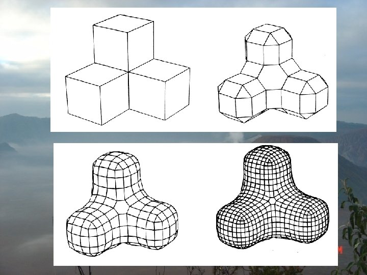
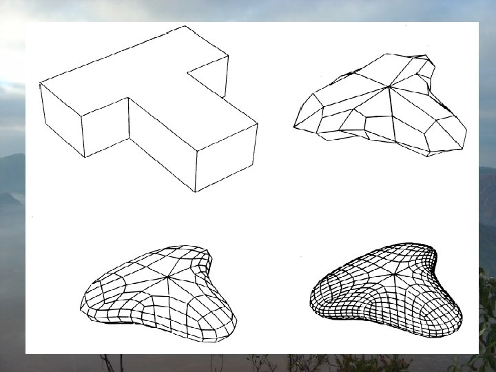
Classification • Vertex insertion (primal) – Insert a vertex on the interior of each edge and one on the interior of each face for quads – Loop, Kobbelt, Catmull-Clark, Modified Butterfly • Corner cutting (dual) – Insert a face in the middle of each old face and connect faces in adjacent old faces – Doo-Sabin

Classification • Interpolating – Can control the limit surface in a more intuitive manner – Can simplify algorithms (efficient) • Approximating – Higher quality surfaces – Faster convergence
 Triangular meshes 2) approximating Loop (C interpolating Butterfly (C 1)")
Face split (primal type) Triangular meshes 2) approximating Loop (C interpolating Butterfly (C 1) Quad. meshes Catmull-Clark(C Kobbelt (C 2) 1) Vertex split (dual type) Quad. meshes approximating 1 1 Doo-Sabin (C ) , Midedge (C )
 Sr (u) = X")
Binary Subdivision of B-Spline • Univariate B-Spline : ( ¤) Sr (u) = X dri N r (u ¡ i ); i 2 Z where N r : normalized B-Spline.
 = 1 Partition")
Properties P • • • N r (u ¡ i ) = 1 Partition of unity : i r Positivity : N (u) ¸ 0 r Local support : N (u ¡ i ) = 0 if u 2= [i ; i + r + 1] Continuity : N r (u) 2 C ( r ¡ 1) Recursion : N r (u ¡ i ) = u ¡r i N r ¡ 1 (u ¡ i ) + i + r +r 1¡ u N r ¡ 1 (u ¡ i ¡ 1)
 as a curve over a refined")
Idea behind Subdivision • Rewrite the curve (*) as a curve over a refined knot sequence Z=2: • (*) becomes Sr (u) = X d^rj N r (2(u ¡ j )) j 2 Z =2 • Determine d^jr A single B-Spline can be decomposed into similar BSpline of half the support.
 = crj N r (2(u ¡")
• This results in Nr X (u) = crj N r (2(u ¡ j )); j 2 Z =2 crj where = 2¡ d^rj = ¡ r r+1 2 j X ¢ crj ¡ i dri ; j 2 Z=2 i 2 Z • For example. X r = 2 d^20 = c¡ 2 i d 2 i = ¢¢¢+ (3=4)d¡ 2 1 + (1=4)d 20 + ¢¢¢ i 2 Z d^21=2 = ¢¢¢+ (1=4)d¡ 2 1 + (3=4)d 20 + ¢¢¢ Chaikin’s algorithm
 = X dri ; s N")
Tensor Product B-Spline Surface Sr ; s (u) = X dri ; s N r ; s (u ¡ i) i 2 Z 2 A tensor product B-Spline is the product of two independently univariate B-Splines, i. e N r ; s (u ¡ i) = N r (u ¡ i )N s (v ¡ j )

d^rj ; s = X r ; s 2 crj ; s d ¡ i i ; j 2 Z =2 i 2 Z 2 crj ; s • • = cri csj = 2¡ ( r + s) µ ¶µ ¶ r + 1 s+ 1 2 i 2 j r = s= 2 9 3 ¢¢¢+ ( )d¡ 2; 21; ¡ 1 + ( ) + d 2; 2 ¢¢¢ 0; ¡ 1 + 16 16 3 1 ¢¢¢+ ( )d¡ 2; 21; 0 + ( ) + d 2; 2 ¢¢¢ 0; 0 + 16 16 The mask set : Example 1 = d^2; 2 0; 0

• Example 2 r = s= 3 The mask for bi-cubic tensor product B-Spline
 Sr ; s; t")
Triangular Spline • A triangular spline surface : ( ¤) Sr ; s; t (u) = X dri ; s; t N r ; s; t (u ¡ i); u 2 R 2; i 2 Z 2 i where N r ; s; t (u) : a normalized triangular spline of degree (r+s+t-2)
 can be rewritten over the refine")
Subdivision of Triangular Spline • The surface (*) can be rewritten over the refine grid. Sr ; s; t (u) = X d^jr ; s; t N r ; s; t 2(u ¡ j ) j • A single triangular spline is decomposed into splines of identical degree over the refined grid. N r ; s; t (u) = X j 2 Z =2 crj ; s; t N r ; s; t (2(u ¡ j ));

d^rj ; s; t = X crj ¡; s; ti dri ; s; t i 2 Z Where crj ; s; t = 2¡ ( r + s+ t ) Xt µ k= 0 r 2 i ¡ k ¶µ ¶µ ¶ s t k 2 j ¡ k The subdivision masks for the triangular spline N 2; 2; 2 (u)

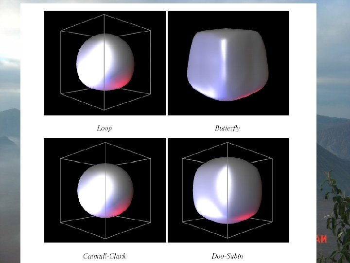
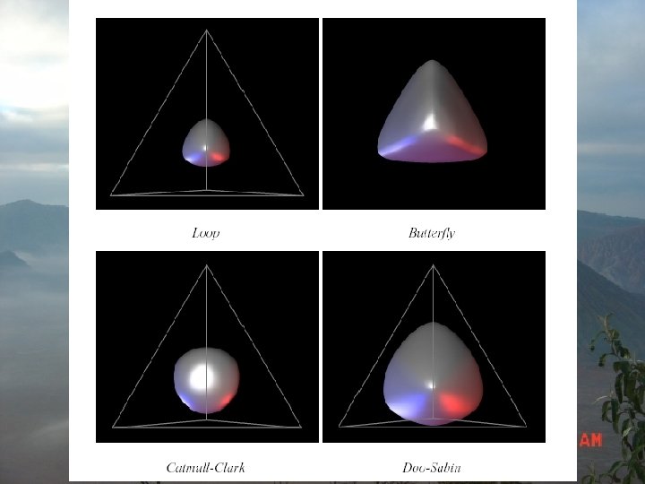
Doo-Sabin Scheme • Approximating Scheme • Tensor Product Quadratic B-Spline • Continuity – C 1 regular regions and extraordinary vertices • Dual Quadrilateral

Doo/Sabin algorithm Problem Subdivision for tensor product quadratic B-spline surface has rigid restrictions on the topology. Each vertex of the net must order 4. This restriction makes the design of many surfaces difficult Doo/Sabin presented an algorithm that eliminated this restriction by generalizing the bi-quadratic B-Spline subdivision rules to include arbitrary topologies.

P’ 3 P 0 P’’ 0 P 3 P’’ 3 (P 0 ; P 1 ; P 2 ; P 3 ) T = S 4 D S (P 0 ; P 1 ; P 2 ; P 3 ) T P’ 0 P’ 2 P’b 2 P’’ 1 P’’ 2 P’ 1 Doo-Sabin Scheme S 4 D S P 2 9 1 6 6 3 = 16 4 1 3 3 9 3 1 1 3 9 3 3 3 1 7 7 3 5 9

• The subdivision masks for bi-quadratic B-Spline : • Geometric view of bi-quadratic B-Spline subdivision : the new points are centroids of the sub-face formed by the face centroid, a corner vertex and the two midedge points next to the corner. arbitrary topology

• For an n-sided face Doo/Sabin used subdivision matrix Sn. D S = (®i j ) n £ n ; ®i j = = 5+ n ; 4 n 3 + 2 cos i= j ³ 4 n 2¼( i ¡ j ) n ´ ; 6 j i= • As subdivision proceeds, the refined control point mesh becomes locally rectangular everywhere except at a fixed number of points. • Since bi-quadratic B-splines are C 1 , the surfaces generated by the Doo/Sabin algorithm are locally C 1

Maple Code: • http: //www. mrl. nyu. edu/projects/subdivision/mapl e/doosabin. pdf

Catmull-Clark Scheme • Approximating Scheme • Tensor Product Bicubic B-spline • Continuity - C 2 regular regions – C 1 extraordinary vertices • Primal Quadrilateral

Catmull/Clark Algorithm P 42 P 41 x x P 31 P 43 x x x P 21 x x x P 33 q 22 x q 11 P 11 x x q 12 x x x P 22 x x x P 32 x P 44 P 23 x x P 34 x x P 24 x P 13 P 12 q 11 : New face points q 12 : New edge points q 22 : New vertex points P 14

• New face points : q 11 = P 11 + P 12 + P 21 + P 22 4 • New edge points : q 12 = C+ D 2 + P 1 2 + P 2 2 ; C = q 11 ; D = q 13 • New vertex points : q 22 = Q R P 22 + + 4 2 4 q 11 + q 13 + q 31 + q 33 4 ·µ ¶ µ ¶ µ ¶¸ 1 p 22 + p 12 p 22 + p 21 p 22 + p 32 p 22 + p 23 + + + R= 4 2 2 Q=

• The subdivision masks for bi-cubic B-Spline : Approach : generalization of bi-cubic B-Spline arbitrary topology

• New face points : the average of all of the old points defining the face. • New edge points : the average of the mid points of the old edge with average of the two new face. 1 Q 4 + 1 R 2 + 1 S; 4 • New vertex points : Q : the average of the new face points of all faces sharing an old vertex point. R : the average of the midpoints of all old edges incident on the old vertex point. S : the old vertex point.

Note : tangent plane continuity was not maintained at extraordinary points. 1 2 N ¡ 3 Q+ S^ = R+ S N N : order of the vertex tangent plane continuity at extraordinary points.

Maple Code: • http: //www. mrl. nyu. edu/projects/subdivision/mapl e/catmullclark. pdf

Butterfly Scheme • Interpolating Scheme • General Scheme • Continuity – C 1 regular regions • Primal Triangular Quadrisection

Butterfly scheme X 1 k k k qe = (pe; 1 + pe; 2 ) + 2 w(pe; 3 + pe; 4 ) ¡ w pe; j 2 = 8 j pki + 1 = pki [ qek 5

The mask of the butterfly scheme:

The mask of the butterfly scheme:

Well-known Fact On the three directional grid, if the values given are constant in one of the three grid directions (1, 0), (0, 1), (1, 1), then the butterfly scheme inserts new values which are constant in the same direction and could be computed by univariate 4 point scheme along the other two grid directions. For a new vertex in the (1, 0) direction, the rule is f 2 ik ++ 11; j = ¡ 1 k (f i ; j + f ik+ 1; j ) + 2 w(f ik+ 1; j + 1 + f ik; j ¡ 1 ) 2 w(f ik+ 2; j + 1 + f ik¡ 1; j ¡ 1 + f ik+ 1; j ¡ 1 )
 f k+ 1")
• For a new vertex in the direction (0, 1) f k+ 1 i ; 2 j + 1 1 k (f i ; j + f ik; j + 1 ) + 2 w(f ik+ 1; j + 1 + f ik¡ 2 w(f ik+ 1; j + 2 + f ik+ 1; j + f ik¡ 1; j ¡ 1 + f ik¡ = ¡ 1; j ) 1; j + 1 ) • For (1, 1) f k+ 1 2 i + 1; 2 j + 1 = ¡ 1 k (f i ; j + f ik+ 1; j + 1 ) + 2 w(f ik+ 1; j + f ik; j + 1 ) 2 w(f ik+ 2; j + 1 + f ik+ 1; j + 2 + f ik¡ 1; j + f ik; j ¡ 1 ) • Under the assumption k f ik; j = f 0; j

• We get from the first insertion rule k f 2 ik ++ 11; j = f 0; j • For a new vertex (0, 1) direction we get +1 = ( f ik; 2 j +1 1 k + f k k k + w)(f 0; j ¡ + w(f f ) 0; j + 1 0; j + 2 0; j ¡ 1 ) 2 • The third insertion rule gives the same rule as above.

Maple Code: • http: //www. mrl. nyu. edu/projects/subdivision/mapl e/butterfly. pdf

Loop Scheme • Approximating Scheme • Three Directional Box-Spline • Continuity – C 2 regular regions – C 1 extraordinary vertices • Primal Triangular Quadrisection

Loop Scheme • A generalized triangular subdivision surface. • The subdivision masks for N 2; 2; 2 (u) • mask A generates new control points for each vertex • mask B generates new control points for edge of the original regular triangular mesh.

• Mask B : generalization is to leave this subdivision rule intact (why? ) • Mask A : The new vertex point can be computed as a convex combination of the old vertex and all old vertices that share an edge with it. 5 3 ^ = V V + Q; 8 8 V : the old vertex point. Q : the average of the old points that share an edge with V. This same idea may be applied to an arbitrary triangular mesh.

• Note : tangent plane continuity is lost at the extraordinary points.
Q; V")
• Loop scheme ^ = ®N V + (1 ¡ ®N )Q; V where ®N = µ ¶ 2 3 1 2¼ 3 + cos + 8 4 N 8 - curvature continuity at regular point. - tangent plane continuity at extaordinary point.

Maple Code • http: //www. mrl. nyu. edu/projects/subdivision/mapl e/loop. pdf

Mid-Edge Scheme P’ 3 P 0 P 3 P’’ 0 P’ 2 P’’ 1 P 1 S 4 M E • For an n-sided face, subdivision matrix : Sn. M E = (¯i j ) n £ n ; P’’ 2 P’ 1 (P 0 ; P 1 ; P 2 ; P 3 ) T = S 4 M E (P 0 ; P 1 ; P 2 ; P 3 ) T 2 3 2 1 0 1 7 16 1 2 1 0 6 7 = 4 4 0 1 2 1 5 1 0 1 2 P 2 1 + cos 2¼( ni ¡ ¯i j = n 1)

Circulant matrix 2 a 0 6 an ¡ 1 6 Sn. G = 6. . 4. a 1 ¢¢¢ an ¡ 2. . . ¢¢¢ a 0 a 1 a 0. . . a 2 3 7 7 7 5 G eigenvalues of Sn can be calculated by evaluating the polynomial. Pn (z) = a 0 + a 1 z + ¢¢¢+ an ¡ 1 zn ¡ 1 ; z = wj ; w= e i 2¼ n ; j = 0; 1; ¢¢¢ ; n ¡ 1

Further Subdivision Schemes • • Non-uniform scheme. Shape preserving scheme. Hermite-type scheme. Variational scheme. Quasi-linear scheme. Poly-scale scheme. Non-stationary scheme. Reverse subdivision scheme.

Convexity Preserving ISS • A constructive approach is used to derive convexity preserving subdivision scheme. f 2 ik + 1 = f 2 ik ++ 11 = f ik ¢ ¡ k ¢ 1¡ k k k f i + 1 ¡ F 1 f i ¡ 1 ; f i + 2 2 1. interpolatory. 2. local : four points scheme. define the first and second differences. df i di = = f i+ 1 ¡ f i d 2 f i = f i + 1 ¡ 2 f i + f i ¡ 1

f 2 ik + 1 = f 2 ik ++ 11 = f ik µ ¶ ¡ ¢ 1 k f i + f ik+ 1 ¡ F 2 (f i + f ik+ 1 ); df ik ; dki+ 1 2 2 3. invariant under addition of affine functions. (★) f 2 ik + 1 = f 2 ik ++ 11 = F f ik ¢ 1¡ k k f i + 1 ¡ F (dki ; dki+ 1 ) 2 : subdivision function 4. continuous 5. homogeneous, i. e. , F (¸ x; ¸ y) = ¸ F (x; y) 6. symmetric
 A subdivision scheme of type (*) satisfying conditions 1")
• Theorem 1 (Convexity) A subdivision scheme of type (*) satisfying conditions 1 to 6 is convex preserving for all convex data F satisfies 0 · F (x; y) · Note : if F=0 1 minf x; yg; 8 x; y ¸ 0 4 linear SS. only C 0 (Question) under what conditions, SS(*) with conditions 1 to 6 and convexity condition generate continuously differentiable limit functions. Answer
 Under the same conditions hold as in Theorem 1.")
• Theorem 2 (Smoothness) Under the same conditions hold as in Theorem 1. The scheme given by f 2 ik + 1 = f 2 ik ++ 11 = f ik ¢ 1 1¡ k k f i + f i+ 1 ¡ 2 4 1 d ki 1 + dk 1 i+ 1 continuously differentiable function which is convex and interpolate the data • Theorem 3 (Approximation order) The convexity preserving subdivision scheme has approximation order 4.

Analysis of convergence and smoothness of binary SS by the formalism of Laurent polynomials A binary univariate SS: f ik + 1 = X ai ¡ 2 j f jk j 2 Z The general form of an interpolatory SS: f 2 ik + 1 = f 2 ik ++ 11 = f ik X j 2 Z a 1+ 2 j f ik¡ j
 = X ai zi i")
For each scheme S, we define the symbol a(z) = X ai zi i 2 Z Theorem 1 Let S be a convergent SS, then ( ¤) X a 2 j = j 2 Z a(¡ 1) = 0; X a 2 j + 1 = 1 j 2 Z a(1) = 2 Theorem 2 Let S denote a SS with symbol a(z) satisfying (*). Then there exists a SS S 1 with the property df k = S 1 df k¡ 1 k k k where f k = Sk f 0 and df = f (df ) i = 2 (f i + 1 ¡ f i )g

Theorem 3 S is a uniformly convergent SS, if only if 1 S 2 1 converges uniformly to the zero function 1 k lim ( S 1 ) f k! 1 2 Theorem 4 Let a(z) = m (R) Sa 1 f 0 2 Cthen convergent, . 0 = 0 ( 1+ z) m 2 m b(z). If Sb is for anyf 0 initial data

Draft Objective: obtain the mask of interpolatory subdivision schemes (binary 2 n-point scheme, ternary 4 -point scheme, butterfly scheme) using symmetry and necessary condition for smoothness. • A binary univariate SS: f ik + 1 = X ai ¡ 2 j f jk j 2 Z The general form of an interpolatory SS: f 2 ik + 1 = f 2 ik ++ 11 = f ik X j 2 Z a 1+ 2 j f ik¡ j

4 -point interpolatory SS • The 4 –point interpolatory SS: f 2 ik + 1 f 2 ik ++ 11 = = f ik a 3 f ik¡ 1 + a 1 f ik + a¡ 1 f ik+ 1 + a¡ 3 f ik+ 2 • The Laurent-polynomial of this scheme is a(z) = a¡ 3 z¡ 3 + a¡ 1 z¡ 1 + a 1 z + a 3 z 3 • By symmetry and necessary condition, we get mask a 1 + a 3 = 1 2 [¡ w; 12 + w; ¡ w]

6 -point interpolatory SS • The 6 –point interpolatory SS: f 2 ik + 1 f 2 ik ++ 11 = = f ik a 5 f ik¡ 2 + a 3 f ik¡ 1 + a 1 f ik + a¡ 1 f ik+ 1 + a¡ 3 f ik+ 2 + a¡ 5 f ik+ 3 • The Laurent-polynomial of this scheme is a(z) = a 5 z¡ 5 + a¡ 3 z¡ 3 + a¡ 1 z¡ 1 + a 1 z + a 3 z 3 + a¡ 5 f ik+ 3 • By symmetry and necessary condition, we get mask a 1 + a 3 + a 5 = 24 a 5 + 8 a 3 + 1 2 = 0 [w; ¡ 1 16 9 + 2 w; ¡ ¡ 3 w; 16 16 1 16 ¡ 3 w; w]

Ternary interpolatory SS • A ternary SS f k+ 1 i = X ai ¡ 3 j f jk j 2 Z • The general form of an interpolatory SS: f 3 ik + 1 = f 3 ik ++ 11 = f ik X a 1+ 3 j f ik¡ k a 2+ 3 j f ik¡ k j 2 Z f k+ 1 3 i + 2 = X j 2 Z
 = X ai zi i")
For each scheme S, we define the symbol a(z) = X ai zi i 2 Z Theorem 5 Let S be a convergent SS, then ( ¤) X j 2 Z a 3 j = X j 2 Z a 3 j + 1 = X a 3 j + 2 = 1 j 2 z a(e 2 i ¼=3 ) = a(e 4 i ¼=3 ) = 0; a(1) = 3 (**) Let us consider a n-ary convergent scheme. The associated polynomial satisfies the properties. a(1) = n; 2 i p ¼ a(wnp ) = 0; wnp = e n ; p 2 f 1; 2; : : : ; n ¡ 1 g
 satisfying (*). Then there")
Theorem 6 Let S denote a SS with symbol a(z) satisfying (*). Then there exists a SS S 1 with the property df k = S 1 df where f k = Sk f 0 and df k¡ 1 k = f (df k ) i = 3 k (f ik+ 1 ¡ f ik )g Theorem 7 S is a uniformly convergent SS, if only if 1 S converges uniformly to the zero function 3 1 1 lim ( S 1 ) k f k! 1 3 0 = 0

Ternary 4 -point interpolatory SS • The ternary 4 –point interpolatory SS: f 3 ik + 1 f 3 ik ++ 11 = = f ik a 4 f ik¡ 1 + a 1 f ik + a¡ 2 f ik+ 1 + a¡ 5 f ik+ 2 f 3 ik ++ 12 = a 5 f ik¡ 1 + a 2 f ik + a¡ 1 f ik+ 1 + a¡ 4 f ik+ 2 • The Laurent-polynomial of this scheme is a(z) = a¡ 5 z¡ 5 + a¡ 4 z¡ 4 + a¡ 2 z¡ 2 + a¡ 1 z¡ 1 + a 1 z + a 2 z 2 + a 4 z 4 + a 5 z 5

• By symmetry and necessary condition, we get mask • Let a 5 = ¡ f 3 ik ++ 11 f 3 ik ++ 12 a 1 + a 2 + a 4 + a 5 3 a 2 ¡ 3 a 4 + 6 a 5 = = 1 1 a 4 + a 5 = 1 ¡ 9 1 18 + 1¹ 6 1 ¡ 18 1 + : [¡ 18 : [¡ 1 13 + ¹; 6 18 1 7 ¡ ¹; 2 18 1 13 + ¹; 2 18 1 ¹ ; ¡ 2 1 + 18 1 ¡ 18 1 ¹] 6

Butterfly subdivision scheme 2 6 6 = A 6 6 4 ¢ ¢ ¡ w ¢ 2 w ¢ ¡ w 2 w 1 2 2 w ¡ w ¢ 2 w 1 2 1 2 1 2 2 w ¢ ¡ w ¢ ¢ ¢ ¡ w ¢ ¢ 3 7 7 7 7 5

• The bivariate Laurent polynomial of this scheme: a(z 1 ; z 2 ) = X 3 ai ; j z 1 i z 2 j i= ¡ 3 j = ¡ 3 • The symbol of the butterfly scheme: a(z 1 ; z 2 ) = c(z 1 ; z 2 ) = + 1 (1 + z 1 )(1 + z 2 )(1 + z 1 z 2 )(1 ¡ wc(z 1 ; z 2 ))(z 1 z 2 ) ¡ 1 ; 2 2 z 1¡ 2 z 2¡ 1 + 2 z 1¡ 1 z 2¡ 2 ¡ 4 z 1¡ 1 z 2¡ 1 ¡ 4 z 1¡ 1 ¡ 4 z 2¡ 1 + 2 z 1¡ 1 z 2 2 z 1 z 2¡ 1 + 12 ¡ 4 z 1 ¡ 4 z 2 ¡ 4 z 1 z 2 + 2 z 12 z 2 + 2 z 1 z 22

• The verification that the scheme generates requires checking the contractivity of three schemes: 2(1 + z 1 )b(z 1 ; z 2 ); 2(1 + z 2 )b(z 1 ; z 2 ); 2(1 + z 1 z 2 )b(z 1 ; z 2 ) • Butterfly scheme satisfies: w ¡ w = 0; w ¡ 2 w + w = 0; ¡ w ¡ 2 w + 1 1 = 0 ¡ + 1¡ 2 2 1 1 ¡ + 2 w + w = 0; 2 2
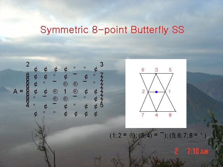

• To converges to a surface with C 0 , we have 2° + ¯ = 0; ¡ 2® + 1 = 0 • This is the same mask of Butterfly scheme: 1; 2 = 1 2 3; 4 = 2 w 5; 6; 7; 8 = ¡ w
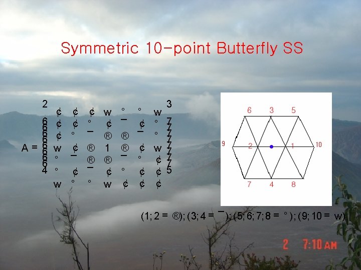

• To converges to a surface with C 0 , we have 2° + ¯ = 0; ¡ 2® ¡ 2 w + 1 = 0 • We find the mask of 10 -point Butterfly scheme: 1; 2 = 1 ¡ w 2 3; 4 = 2° 5; 6; 7; 8 = ¡ ° 9; 10 = w • This mask is exact with a modified Butterfly scheme ° = 1 + w 16

Non-stationary Subdivision Scheme • Construction an insertion rule by interpolation with the span of the functions f 1; t; cost; sin tg • Consider the k-th level insertion rule at the point µ 2¡ k ¡ 1 based on the values at the points ¡ µ 2¡ k ; 0; µ 2¡ k ; 2µ 2¡ k the solution of system leads to the insertion rule f k+ 1 2 i + 1 = + ¡ 1 k k ) + f (f ¡ +2 i i 1 16 cos 2 (µ 2¡ k ¡ 2 ) cos(µ 2¡ k ¡ 1 ) (1 + 2 cos(µ 2¡ k ¡ 1 )) 2 k + f k ) (f i i+ 1 16 cos 2 (µ 2¡ k ¡ 2 ) cos(µ 2¡ k ¡ 1 )

Non-stationary Butterfly Scheme • Objective: given a well-known non-stationary 4 point scheme as the following rule: f 2 ik ++ 11 = + ¡ 1 k k ) + f (f i+ 2 16 cos 2 (µ 2¡ k ¡ 2 ) cos(µ 2¡ k ¡ 1 ) i ¡ 1 (1 + 2 cos(µ 2¡ k ¡ 1 )) 2 k + f k ) (f i+ 1 16 cos 2 (µ 2¡ k ¡ 2 ) cos(µ 2¡ k ¡ 1 ) i • Our objective is to extend this non-stationary 4 point scheme to 2 D Butterfly scheme, we denote wk = 16 cos(µ 2¡ k¡ 1 2 ) cos(µ 2¡ k ¡ 1)

Definition Two SSs f Sa g and f Sbk g are asymptotically k equivalent if X 1 k. Sa k ¡ Sbk k < 1 k= 0 where k. Sa k k 1 = maxf $ S X$ (k) ja 2® j; X (k) ja 2®+ 1 jg Theorem 1 Let f Sa k gand f Sa g be two asymptotically equivalent SSs having finite masks of the same support. Suppose f Sa k gis non-stationary and f Sa g is stationary. If f Sa g is C m and X 1 k= 0 2 m k k. Sa k ¡ Sa k < 1 m Then the non-stationary scheme f Sa k g is C.

Lemma For k ¸ 0; 0 · µ · ¼=2 1 1 · wk · 16 8 jwk ¡ $ S $ 1 C j · 2 k 16 2 The mask of f Sk g : 2 ¢ 6 6 ¡ wk 6 4 ¡ wk ¢ ¢ ¢ ¡ wk ¢ 2 wk ¢ ¡ wk 2 wk 1 2 2 wk ¡ wk ¢ 2 wk 1 2 1 2 1 2 2 wk ¢ ¡ wk ¢ ¢ ¢ ¡ wk ¢ ¢ 3 7 7 7 7 5

Subdivision operator S associated with butterfly scheme has mask: 2 ¢ ¢ ¢ 6 ¢ ¢ ¡ 1=16 6 6 ¢ ¡ 1=16 1=8 6 1 6 ¢ ¢ 6 2 1 6 ¡ 1=16 1=8 6 2 4 ¡ 1=16 ¢ 1=8 ¢ ¡ 1=16 3 ¢ ¡ 1=16 ¢ ¢ ¢ ¡ 1=16 7 1=8 7 1 1 7 ¡ 1=8 1=16 7 2 2 1 7 ¢ ¢ 1 7 2 1 7 ¢ ¡ 1=8 1=16 7 2 ¢ ¡ 1=16 ¢ ¢ 5 ¢ ¢ Theorem The non-stationary butterfly scheme f Sk g is asymptotically equivalent to the stationary butterfly schemef Sg. Moreover, the limit function belong to. C 1
 • Approximating Scheme • Continuity – C 2 regular regions")
p 3 Subdivision (Kobbelt) • Approximating Scheme • Continuity – C 2 regular regions – C 1 extraordinary vertices • Triangular Trisection • Adaptive Refinement

p 3 Subdivision • Subdivision schemes on triangle meshes are usually based on the 1 -to-4 split operation which inserts a new vertex for every edge of the given mesh and then connects the new vertices.

p 3 Subdivision • This scheme is based on a split operation which first inserts a new vertex for every face of the given mesh. Flipping the original edges. Applying this scheme twice leads to a 1 -to-9 refinement of the original mesh.

Smoothing Rules • Two smoothing rules, one for the placement of the newly inserted vertices and one for the relaxation of the old ones. • Reverse Engineering Process: instead of analyzing a given scheme, we derive one which by construction satisfies the known necessary criteria. q : = 1 (p + pj + pk ) 3 i n¡ 1 1 X S(p) : = (1 ¡ ®n )p + ®n pi n = i 0

Subdivision Matrix • When analyzing the eigen-structure of this matrix, it is not suitable all eigenvalues are complex 2 u v. 6 1 1 6 6 1 0 16 6 S= 6. . 3 6. . 6 6 4 1 0 1 1 v 1. . . 0 ¢¢¢. . . . ¢¢¢ 0 v 0. . . 3 7 7 7 0 7 7 7 1 5 1 u = 3(1 ¡ ®n ); v = 3®=n

Subdivision Matrix 2 The matrix S~ = RS has its eigen-values: 1 1 n¡ 1 [9; (2 ¡ 3®n ) 2 ; 2 + 2 cos(2¼ ); ¢¢¢ ; 2 + 2 cos(2¼ )] 9 n n The necessary condition for C 1: . ¸ 1 = 1 > ¸ 2 = ¸ 3 > ¸ i ; i = 4; : : : ; n + 1 The choice for the eigen-values: ¸ 4 = ¸ 2 2 ) ®n = 4 ¡ 2 cos(2¼=n) 9 2 1 6 0 6 6 = R 6 6 0 6. . 4. 0 3 0 ¢¢¢ 0 0 0 ¢¢¢ 0 1 7 7 7. . 1. . 0 7 7. . . . 7. 5. . . 0 1 0

Boundaries • Edge flipping at the boundaries is not possible. • We have to apply a univariate tri-section rule to the boundary polygon and connect the new vertices to the corresponding interior ones such that a uniform 1 -to-9 split is established for each boundary triangle. • We can obtain tri-section mask for cubic splines by convolution 1 1 1 2 = ¤ [1; 2; 3; 2; 1] ( [1; 1; 1]) [1; 4; 10; 16; 19; 16; 10; 4; 1] 3 3 27

Interpolatory p 3 -Subdivision Stencil for a new vertex and scheme: qk + 1 = 32 k 1 k 2 k k k (p 1 + p 2 + p 3 ) ¡ (p 4 + p 5 + p 6 ) ¡ (p 7 + pk 8 + pk 9 + pk 10 + pk 11 + pk 12 ) 81 81 81

Interpolatory p 3 -Subdivision Modification for extraordinary vertices: qk + 1 = ®pk + n X¡ 1 ®i pki i= 0 For n ¸ 5 8 = ® ; 9 ®in = For n= 3 For n= 4 1 9 + 2 3 cos(2¼i =n) + n 2 9 cos(4¼i =n) ¡ 2 8 7 ; ® 0 = ; ® 1 = ® 2 = 9 27 27 ¡ 5 8 7 1 ® = ; ® 0 = ; ® 1 = ® 3 = ; ® 2 = 9 36 27 36 ®=

• Stencil for boundary subdivision k+ 1 = ¡ p 3 i ¡ 1 4 k p 81 i ¡ 2+ 10 k p 27 i ¡ 1+ 20 k 5 k pi ¡ p 27 81 i + 1 pk 3 i = pki k+ 1 = ¡ p 3 i +1 5 k pi ¡ 81 1+ 20 k 10 k 4 k pi + 1 ¡ pi + 2 27 27 81

• Reflection vertices across the boundary of the mesh

Eigen Structure of SS • Successive applying of a matrix relates to eigenvectors and values. • Applying of a matrix to a vector produces a transformation on the vector Sv = ¸ v • Why are eigenvalues and vectors so important? Sv; S 2 v; S 3 v; : : : ¸ v; ¸ 2 v; ¸ 3 v; : : : same limit

Affine Invariance Sum of row elements must be unit, so 2 6 6 S 6 4 1 1. . . 1 3 2 7 6 7= 6 7 6 5 4 1 1. . . 3 7 7 7 5 1 • What is the interpretation of above relation? 2 6 6 1= 6 4 1 1. . . 1 3 7 7 7 5 is an eigenvector of S and ¸ = 1 is the corresponding eigenvalue

Subdivision Limit Position • If 1 = ¸ 0 > ¸ i ; f i = 1; ng ¸ 0 S = = V¤V¡ £ v 0 1 v 1 then S is C 0. 2 ¢¢¢vn ¤ 6 6 6 4 ¸ 0 0. . . 0 ¸ 1. . . 0 0 ¢¢¢ 0. . . ¢¢¢ ¸ n 32 76 76 76 54 v 0¡ 1 v 1¡ 1. . . vn¡ 1 3 7 7 7 5

• To find the limit neighborhood P 1 , we must compute S 1 = = V¤ 1 V¡ £ 1 v 1 1 2 ¢¢¢vn ¤ 6 6 6 4 32 v 0¡ 1 v 1¡ 1 1 0 ¢¢¢ 0 6 0 0 ¢¢¢ 0 7 76. . . . 7 6. . 54. . . 0 0 ¢¢¢ 0 vn¡ 1 3 2 P 1 v 0¡ 1 3 6 7 7 P 0 = S 1 P 0 = 6 4 ¢¢¢ 5 v 0¡ 1 3 7 6 7 7= 6 7 7 4 ¢¢¢ 5 5 v 0¡ 1 All of the vertices of the limit local neighborhood converges to the same position 2 v 0¡ 1

Subdivision Derivatives The 1 st derivatives of the subdivision manifold for a parameter direction u defines: @S 1 pgi+ 1 ¡ pgi = lim g 0 g ! 1 ¸ kp 0 @u 1 i + 1 ¡ pi k We define the 2 nd and 3 rd derivatives @2 S 1 (pgi+ 1 ¡ pig ) ¡ (pgi ¡ pgi¡ 1 ) = lim g 0 0 k 2 2 g! 1 ¸ ¡ @u p kp 2 i+ 1 i @3 S 1 (pig+ 2 ¡ 2 pgi+ 1 + pig ) ¡ (pgi+ 1 ¡ 2 pig + pgi¡ 1 ) = lim g 0 0 k 3 3 g! 1 ¸ ¡ @u p kp 3 i+ 1 i

Example: Uniform Cubic Spline • Eigen Decomposition of S: 2 6 16 S= 6 86 4 2 6 6 4 1 0 0 1 4 6 4 1 1 ¡ 1=2 2=11 ¡ 1=11 1 0 1 1=2 2=11 1 0 0 1 4 6 0 0 1 1 0 0 3 2 7 7 7 = V¤V¡ 7 5 6 6 4 0 0 1 3 2 7 7 5 6 6 4 1 1 0 0 0 1=2 0 0 0 1=4 0 0 0 0 0 1=8 0 1=6 4=6 1=6 0 0 ¡ 1 0 0 11=6 ¡ 22=6 11=6 0 ¡ 1 0 1 ¡ 3 3 ¡ 3 1 0 ¡ 1 3 3 7 7 7 7 5

Sg = = 2 6 6 6 g 6 = S 6 6 4 6¸ 3 g 6 0 0 V ¤ 2 g V ¡ 1 6 0 6 V 6 6 0 4 0 0 1 0 ¸ g 1 0 0 0 1+ 6¸ 1 g + 11¸ g 2 ¡ 18¸ g 3 6 1+ 3¸ 1 g + 2¸ g 2 6 1¡ 6¸ 1 g + 11¸ g 2 ¡ 6¸ g 3 6 0 0 ¸ g 2 0 0 0 0 0 ¸ g 3 4¡ 22¸ g 2 + 18¸ 6 4¡ 4¸ g 2 6 4+ 2¸ g 2 6 4¡ 4¸ g 2 6 4¡ 22¸ g 2 + 18¸ 6 g 3 3 7 7 7 V¡ 7 5 1 1¡ 6¸ g 1 + 11¸ g 2 ¡ 6¸ g 3 6 1¡ 3¸ g 1 + 2¸ g 2 6 1¡ ¸ g 2 6 1+ 3¸ g 1 + 2¸ g 2 6 1+ 6¸ g 1 + 11¸ g 2 ¡ 18¸ g 3 6 0 0 6¸ g 3 6 3 7 7 7 5

Limit Position • We derive the formula for the limit position 2 S 1 6 6 = 6 6 4 0 0 0 1=6 1=6 1=6 4=6 4=6 4=6 1=6 1=6 1=6 0 0 0 3 7 7 5 P 1 = S 1 P 0 V 0; 0; 0 = 1 V¡ 6 2; ¡ 1; 0 + 4 V¡ 6 1; 0; 1 + 1 V 0; 1; 2 6

1 st Derivatives pig+ 1 pgi Differencing and is the same as differencing g + 1 i i S the corresponding row and of 2 ¡ 1 1 0 0 6 0 ¡ 1 1 0 Du = 6 4 0 0 ¡ 1 1 0 0 0 ¡ 1 @Sg = D u Sg @u 2 6 @Sg = 6 6 @u 4 ¡ 2¸ 2 0 0 0 g 3 ¡ ¸ g 1 ¡ 3¸ g 2 + 6¸ 2 ¡ ¸ g 1 ¡ ¸ g 2 2 ¡ ¸ g 1 + 3¸ g 2 ¡ 2¸ 2 3 g 3 6¸ g 2 ¡ 6¸ g 3 2 2¸ g 2 2 ¡ 6¸ g 2 + 6¸ g 3 2 ¸ g 1 ¡ 3¸ g 2 + 2¸ 2 ¸ g 1 ¡ ¸ g 2 2 ¸ g 1 + 3¸ g 2 ¡ 6¸ 2 g 3 0 0 7 7 0 5 1 0 0 0 2¸ g 3 2 3 7 7 7 5

• We derive the subdivision process is C 1: 2 0 6 @S 1 1 @Sg = lim g = 6 0 4 0 g! 1 ¸ @u u 1 @ 0 ¡ ¡ 1 2 1 2 0 0 @P 1 @S 1 0 = P @u @u @V 0; 0; 0 1 = ¡ V¡ u 2 2; ¡ 1 V 1; 0 + 2 0; 1; 2 1 2 1 2 3 0 0 7 7 0 5 0

2 nd Derivatives The same finite differencing can be done to the 1 st derivatives matrix to compute 2 nd derivatives: 2 @2 Sg @Sg = Duu 2 @u @u 2 g 3 ¸ @2 Sg = 4 0 @u 2 0 Duu g 2 g 3 ¸ ¡ 3¸ ¸ g 2 ¡ ¸ g 3 3 ¡ 1 1 0 0 = 4 0 ¡ 1 1 0 5 0 0 ¡ 1 1 g 2 g 3 ¡ 2¸ + 3¸ ¡ 2¸ g 2 + 3¸ g 3 g 2 g 3 ¸ ¡ ¸ ¸ g 2 ¸ 2 g ¡ 3¸ g 3 3 0 0 5 ¸ g 3

• We derive the subdivision process is C 2: 2 3 0 1 ¡ 2 1 0 @2 S 1 1 @2 Sg = lim g = 4 0 1 ¡ 2 1 0 5 2 2 g! 1 ¸ @u u 2 @ 0 1 ¡ 2 1 0 @2 P 1 @2 S 1 0 = P 2 @u @u 2 @2 V 0; 0; 0 = V¡ 2 u 2; ¡ 1; 0 ¡ 2 V¡ 1; 0; 1 + V 0; 1; 2

3 rd Derivatives We can iterate again to check if the subdivision process is C 3: · @3 Sg @2 Sg = Duuu 3 @u @u 2 @3 Sg = 3 @u · ¡ ¸ 0 Duuu = g 3 3¸ g 3 ¡ 1 1 0 0 ¡ 1 1 g 3 ¸ ¡ 3¸ g 3 0 ¸ 3 g ¸ ¸ The rows are not the same, so the process is not C 3

Catmull-Clark Subdivision

Loop Subdivision

p 3 Subdivision
- Slides: 133