The Greedy Approach Young CS 530 Adv Algo

The Greedy Approach Young CS 530 Adv. Algo. Greedy 1

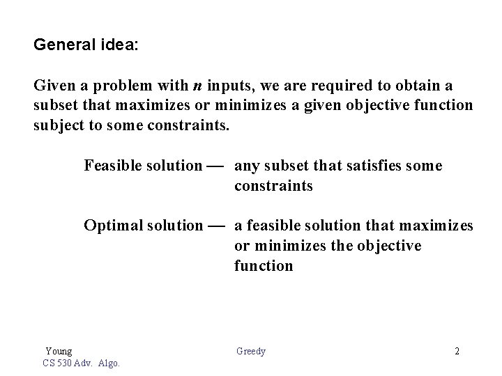
General idea: Given a problem with n inputs, we are required to obtain a subset that maximizes or minimizes a given objective function subject to some constraints. Feasible solution — any subset that satisfies some constraints Optimal solution — a feasible solution that maximizes or minimizes the objective function Young CS 530 Adv. Algo. Greedy 2

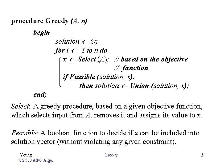
procedure Greedy (A, n) begin solution Ø; for i 1 to n do x Select (A); // based on the objective // function if Feasible (solution, x), then solution Union (solution, x); end; Select: A greedy procedure, based on a given objective function, which selects input from A, removes it and assigns its value to x. Feasible: A boolean function to decide if x can be included into solution vector (without violating any given constraint). Young CS 530 Adv. Algo. Greedy 3

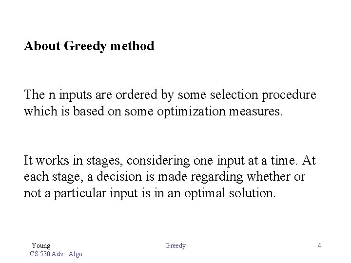
About Greedy method The n inputs are ordered by some selection procedure which is based on some optimization measures. It works in stages, considering one input at a time. At each stage, a decision is made regarding whether or not a particular input is in an optimal solution. Young CS 530 Adv. Algo. Greedy 4

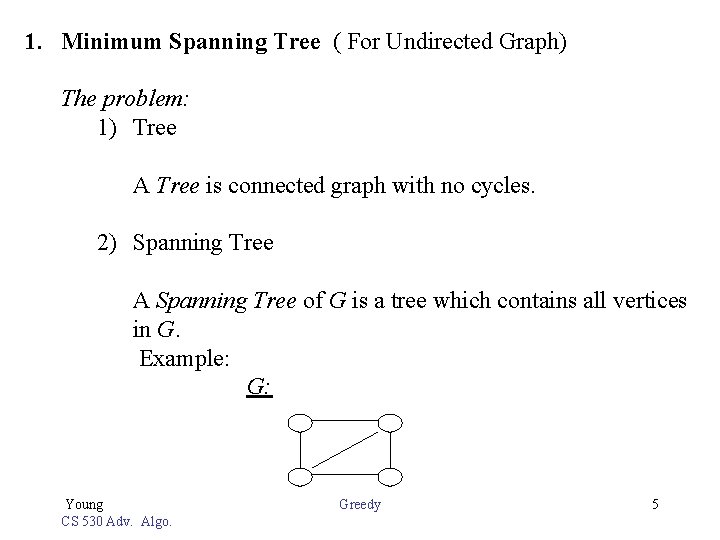
1. Minimum Spanning Tree ( For Undirected Graph) The problem: 1) Tree A Tree is connected graph with no cycles. 2) Spanning Tree A Spanning Tree of G is a tree which contains all vertices in G. Example: G: Young CS 530 Adv. Algo. Greedy 5

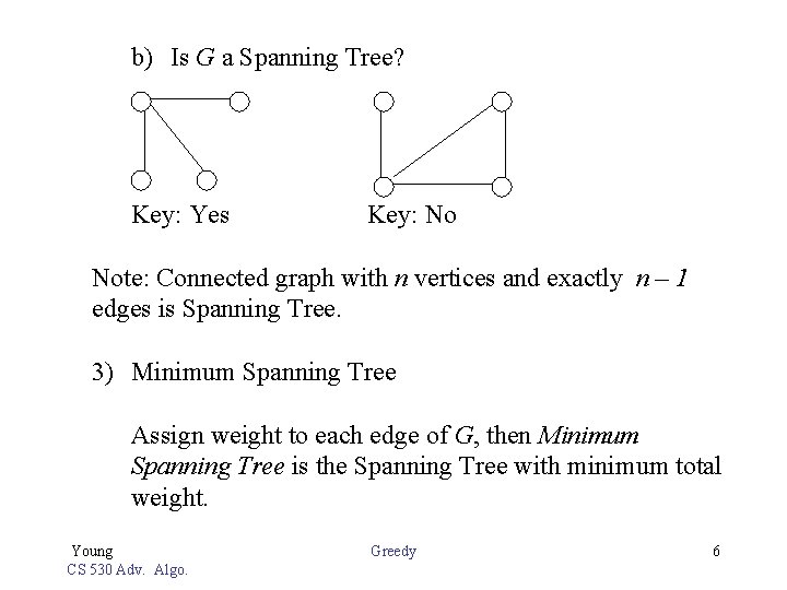
b) Is G a Spanning Tree? Key: Yes Key: No Note: Connected graph with n vertices and exactly n – 1 edges is Spanning Tree. 3) Minimum Spanning Tree Assign weight to each edge of G, then Minimum Spanning Tree is the Spanning Tree with minimum total weight. Young CS 530 Adv. Algo. Greedy 6

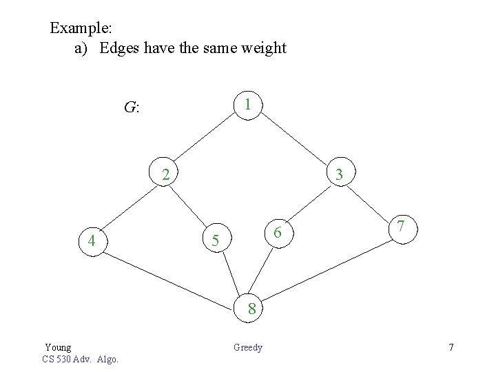
Example: a) Edges have the same weight 1 G: 2 4 3 6 5 7 8 Young CS 530 Adv. Algo. Greedy 7

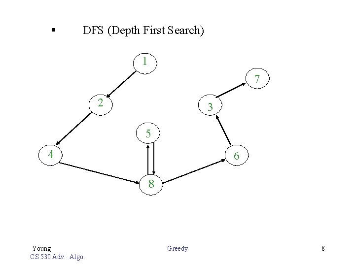
§ DFS (Depth First Search) 1 7 2 3 5 4 6 8 Young CS 530 Adv. Algo. Greedy 8

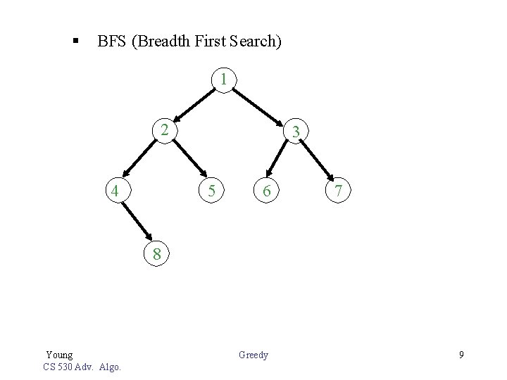
§ BFS (Breadth First Search) 1 2 4 3 5 6 7 8 Young CS 530 Adv. Algo. Greedy 9

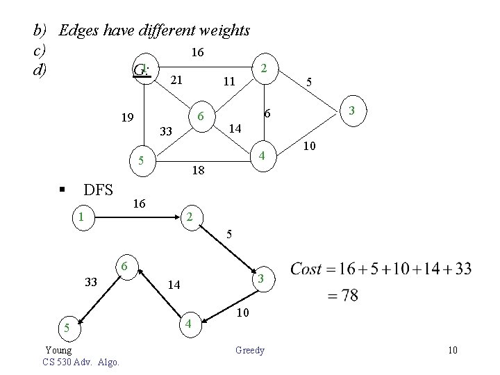
b) Edges have different weights c) 16 1 d) G: 21 11 6 19 33 DFS 3 6 14 10 18 16 1 5 4 5 § 2 2 5 6 33 5 Young CS 530 Adv. Algo. 3 14 4 10 Greedy 10

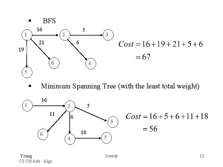
§ BFS 1 16 5 2 21 3 6 19 6 4 5 § Minimum Spanning Tree (with the least total weight) 1 16 5 2 11 6 Young CS 530 Adv. Algo. 6 3 18 4 5 Greedy 11

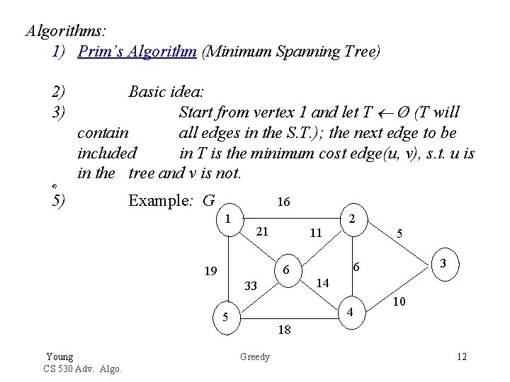
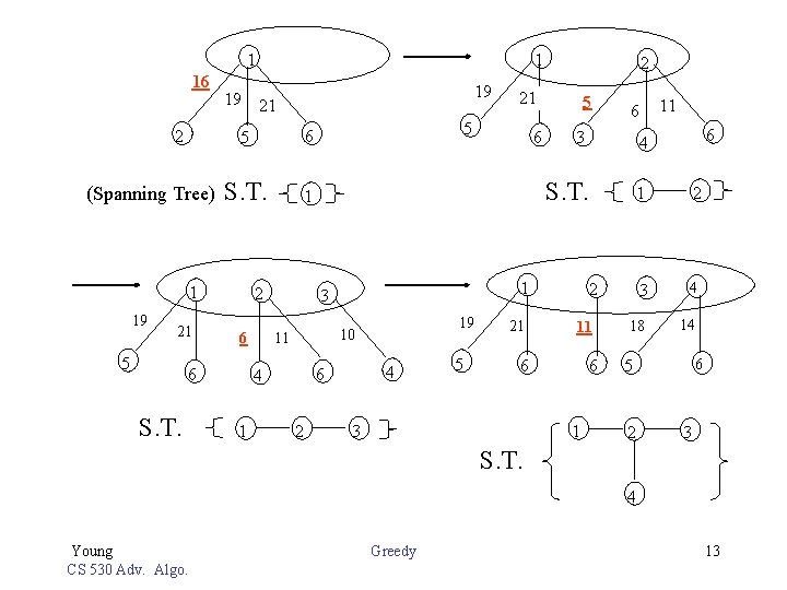
Algorithms: 1) Prim’s Algorithm (Minimum Spanning Tree) 2) 3) Basic idea: Start from vertex 1 and let T Ø (T will contain all edges in the S. T. ); the next edge to be included in T is the minimum cost edge(u, v), s. t. u is in the tree and v is not. 4) 5) Example: G 16 1 21 11 6 19 33 5 3 6 14 4 5 Young CS 530 Adv. Algo. 2 10 18 Greedy 12

1 16 2 (Spanning Tree) 19 21 5 6 S. T. 1 2 1 19 10 4 6 2 6 5 5 21 6 4 S. T. 1 2 3 4 18 14 2 11 6 3 1 3 4 2 21 5 11 6 6 S. T. 19 21 5 1 19 1 6 5 2 3 S. T. 4 Young CS 530 Adv. Algo. Greedy 13

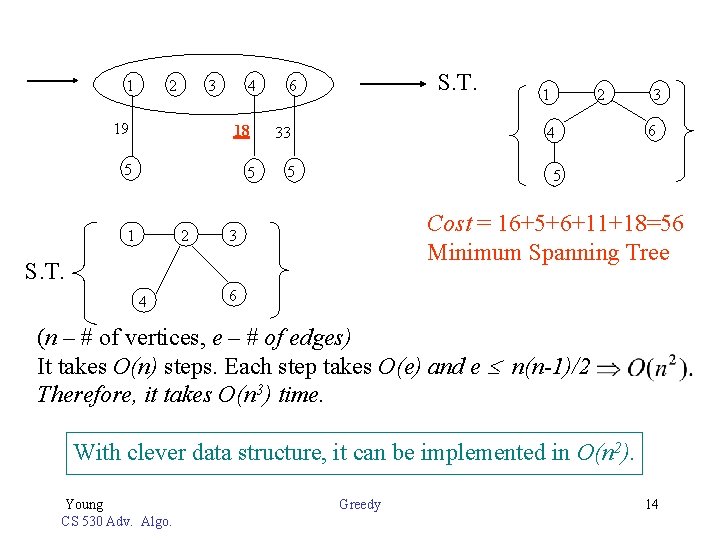
1 2 4 3 19 18 5 5 1 2 S. T. 6 33 2 4 5 3 6 5 Cost = 16+5+6+11+18=56 Minimum Spanning Tree 3 S. T. 4 1 6 (n – # of vertices, e – # of edges) It takes O(n) steps. Each step takes O(e) and e n(n-1)/2 Therefore, it takes O(n 3) time. With clever data structure, it can be implemented in O(n 2). Young CS 530 Adv. Algo. Greedy 14

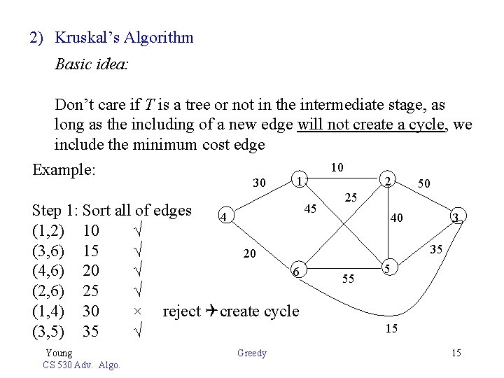
2) Kruskal’s Algorithm Basic idea: Don’t care if T is a tree or not in the intermediate stage, as long as the including of a new edge will not create a cycle, we include the minimum cost edge Example: 30 1 45 Step 1: Sort all of edges 4 (1, 2) 10 √ (3, 6) 15 √ 20 6 (4, 6) 20 √ (2, 6) 25 √ (1, 4) 30 × reject create cycle (3, 5) 35 √ Young CS 530 Adv. Algo. Greedy 10 2 25 50 3 40 35 55 5 15 15

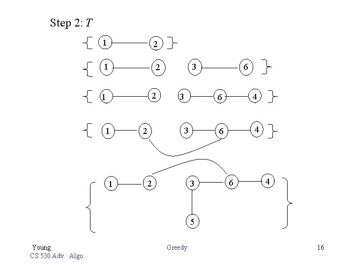
Step 2: T 1 2 2 1 1 1 2 3 6 4 2 3 6 4 5 Young CS 530 Adv. Algo. Greedy 16

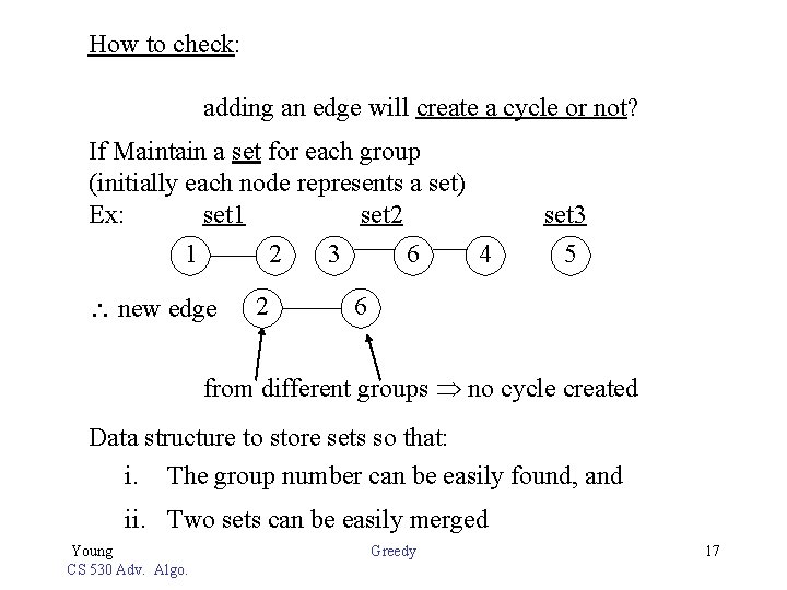
How to check: adding an edge will create a cycle or not? If Maintain a set for each group (initially each node represents a set) Ex: set 1 set 2 1 2 new edge 2 3 6 set 3 4 5 6 from different groups no cycle created Data structure to store sets so that: i. The group number can be easily found, and ii. Two sets can be easily merged Young CS 530 Adv. Algo. Greedy 17

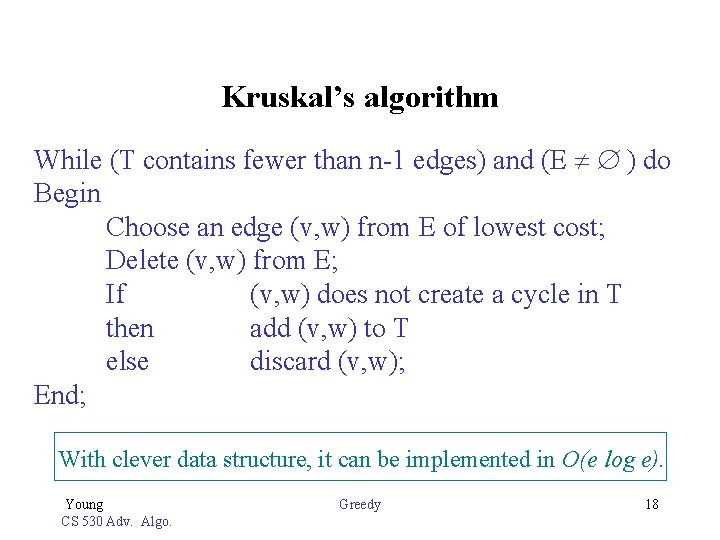
Kruskal’s algorithm While (T contains fewer than n-1 edges) and (E ) do Begin Choose an edge (v, w) from E of lowest cost; Delete (v, w) from E; If (v, w) does not create a cycle in T then add (v, w) to T else discard (v, w); End; With clever data structure, it can be implemented in O(e log e). Young CS 530 Adv. Algo. Greedy 18

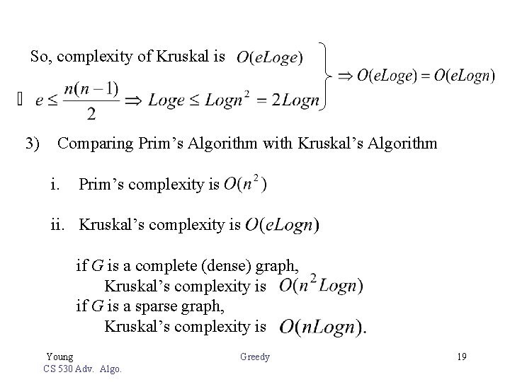
So, complexity of Kruskal is 3) Comparing Prim’s Algorithm with Kruskal’s Algorithm i. Prim’s complexity is ii. Kruskal’s complexity is if G is a complete (dense) graph, Kruskal’s complexity is . if G is a sparse graph, Kruskal’s complexity is Young CS 530 Adv. Algo. Greedy 19

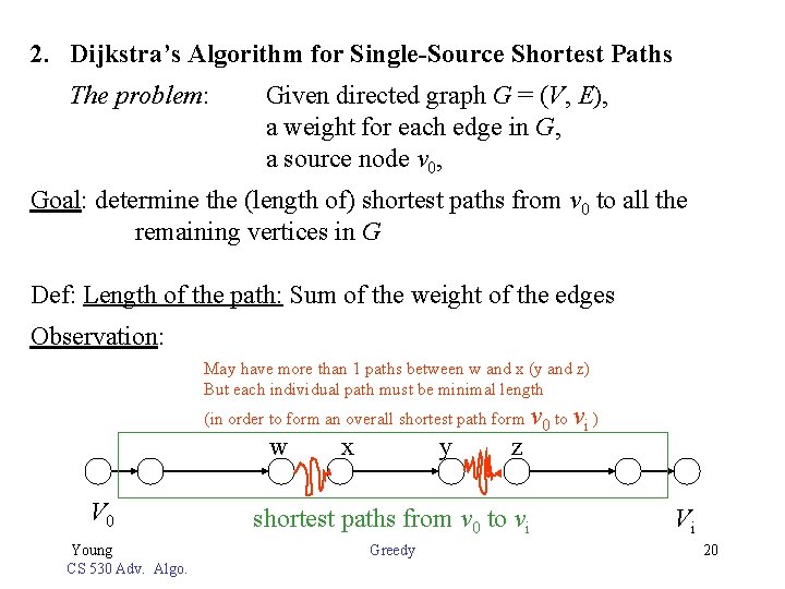
2. Dijkstra’s Algorithm for Single-Source Shortest Paths The problem: Given directed graph G = (V, E), a weight for each edge in G, a source node v 0, Goal: determine the (length of) shortest paths from v 0 to all the remaining vertices in G Def: Length of the path: Sum of the weight of the edges Observation: May have more than 1 paths between w and x (y and z) But each individual path must be minimal length (in order to form an overall shortest path form v 0 to vi ) w x y z V 0 Young CS 530 Adv. Algo. shortest paths from v 0 to vi Greedy Vi 20

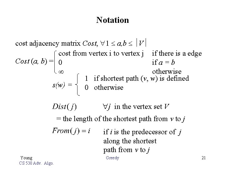
Notation cost adjacency matrix Cost, 1 a, b V cost from vertex i to vertex j if there is a edge Cost (a, b) = 0 if a = b otherwise 1 if shortest path (v, w) is defined s(w) = 0 otherwise in the vertex set V = the length of the shortest path from v to j if i is the predecessor of j along the shortest path from v to j Young CS 530 Adv. Algo. Greedy 21

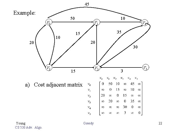
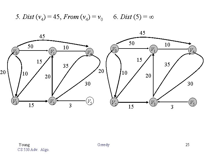
45 Example: 50 V 1 V 4 35 15 10 10 20 20 V 2 V 3 15 30 3 V 5 a) Cost adjacent matrix Young CS 530 Adv. Algo. Greedy 22

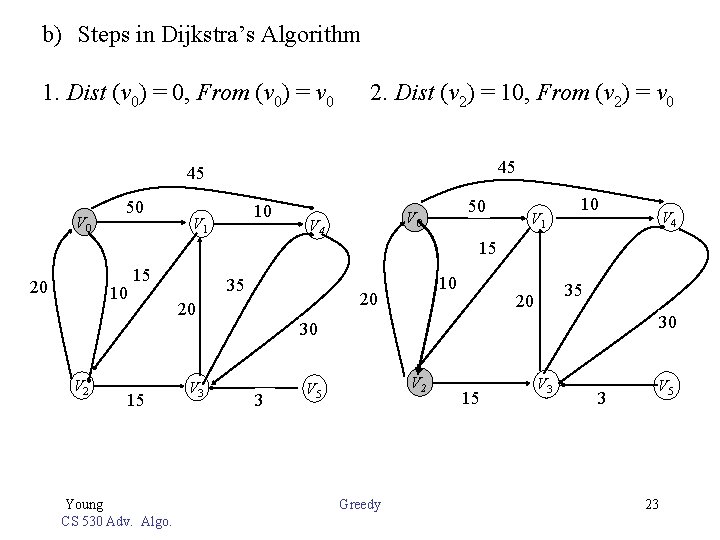
b) Steps in Dijkstra’s Algorithm 1. Dist (v 0) = 0, From (v 0) = v 0 2. Dist (v 2) = 10, From (v 2) = v 0 45 45 V 0 50 10 V 1 50 V 4 V 1 10 V 4 15 20 10 15 35 10 20 20 35 20 30 30 V 2 15 Young CS 530 Adv. Algo. V 3 3 V 2 V 5 Greedy 15 V 3 3 V 5 23

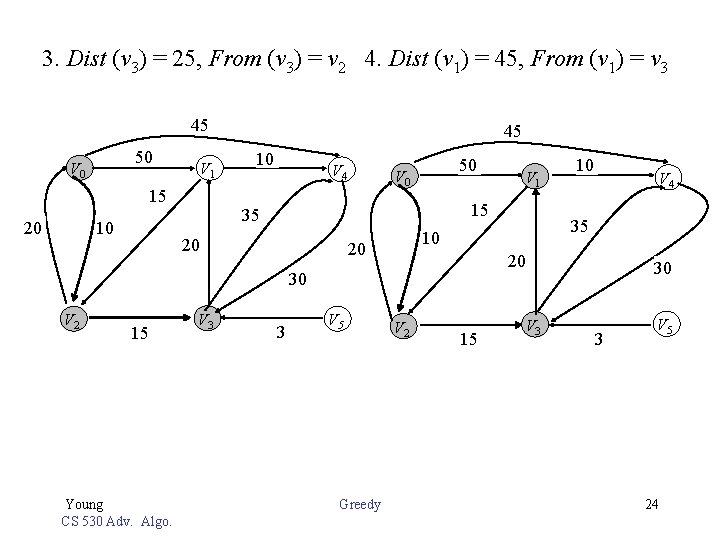
3. Dist (v 3) = 25, From (v 3) = v 2 4. Dist (v 1) = 45, From (v 1) = v 3 45 50 V 1 15 20 10 45 10 V 4 50 V 0 15 35 20 20 15 Young CS 530 Adv. Algo. V 3 3 V 5 Greedy 10 V 4 35 10 20 30 V 2 V 1 V 2 15 V 3 30 3 V 5 24

5. Dist (v 4) = 45, From (v 4) = v 0 6. Dist (5) = 45 45 V 0 50 V 1 15 20 10 10 50 V 4 V 1 15 35 20 20 10 10 V 4 35 20 30 30 V 2 15 Young CS 530 Adv. Algo. V 3 3 V 5 V 2 Greedy 15 V 3 V 5 3 25

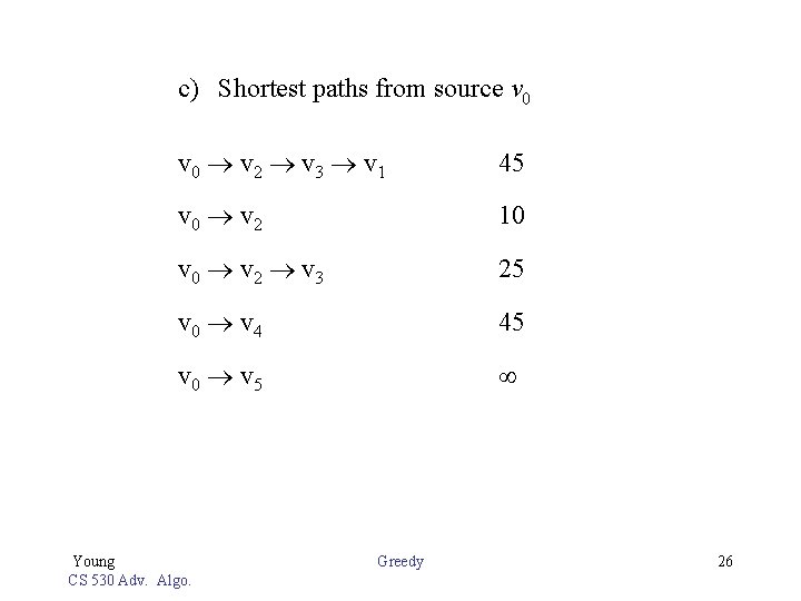
c) Shortest paths from source v 0 v 2 v 3 v 1 45 v 0 v 2 10 v 0 v 2 v 3 25 v 0 v 4 45 v 0 v 5 Young CS 530 Adv. Algo. Greedy 26

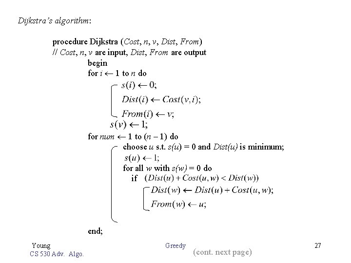
Dijkstra’s algorithm: procedure Dijkstra (Cost, n, v, Dist, From) // Cost, n, v are input, Dist, From are output begin for i 1 to n do for num 1 to (n – 1) do choose u s. t. s(u) = 0 and Dist(u) is minimum; for all w with s(w) = 0 do if end; Young CS 530 Adv. Algo. Greedy (cont. next page) 27

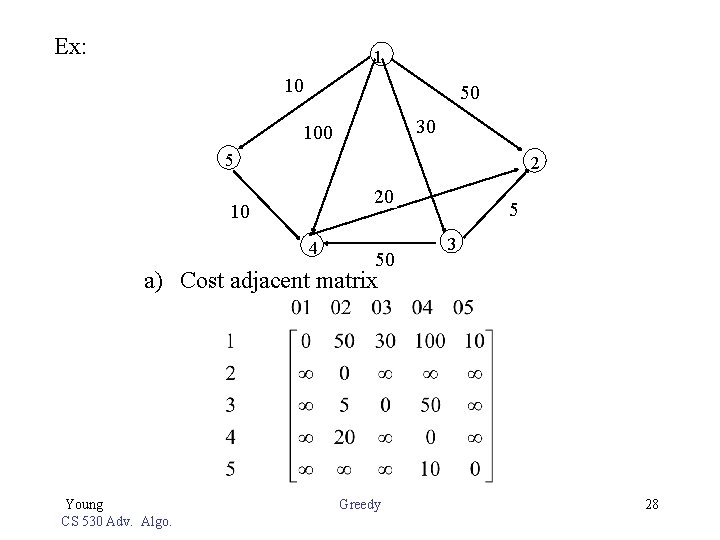
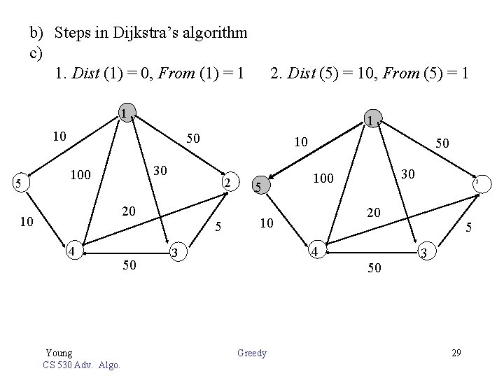
Ex: 1 10 50 30 100 5 2 20 10 4 50 5 3 a) Cost adjacent matrix Young CS 530 Adv. Algo. Greedy 28

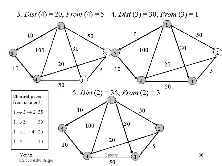
b) Steps in Dijkstra’s algorithm c) 1. Dist (1) = 0, From (1) = 1 2. Dist (5) = 10, From (5) = 1 10 5 50 10 30 100 2 20 10 5 4 Young CS 530 Adv. Algo. 50 5 50 30 100 20 10 4 3 50 Greedy 2 5 3 29

3. Dist (4) = 20, From (4) = 5 4. Dist (3) = 30, From (3) = 1 10 4 50 Shortest paths from source 1 1 5 10 Young CS 530 Adv. Algo. 5 2 20 10 3 4 5. Dist (2) = 35, From (2) = 3 10 30 1 5 4 20 30 50 5 3 1 1 3 2 35 1 3 50 100 2 5 20 10 30 100 5 10 50 5 50 30 100 2 20 10 4 Greedy 50 5 3 30

3. Optimal Storage on Tapes The problem: Given n programs to be stored on tape, the lengths of these n programs are l 1, l 2 , . . . , ln respectively. Suppose the programs are stored in the order of i 1, i 2 , . . . , in Let tj be the time to retrieve program ij. Assume that the tape is initially positioned at the beginning. tj is proportional to the sum of all lengths of programs stored in front of the program ij. Young CS 530 Adv. Algo. Greedy 31

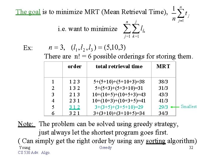
The goal is to minimize MRT (Mean Retrieval Time), i. e. want to minimize Ex: There are n! = 6 possible orderings for storing them. order total retrieval time MRT 1 2 3 4 5 6 1 2 3 1 3 2 2 1 3 2 3 1 2 3 2 1 5+(5+10)+(5+10+3)=38 5+(5+3)+(5+3+10)=31 10+(10+5)+(10+5+3)=43 10+(10+3)+(10+3+5)=41 3+(3+5)+(3+5+10)=29 3+(3+10)+(3+10+5)=34 38/3 31/3 43/3 41/3 29/3 34/3 Smallest Note: The problem can be solved using greedy strategy, just always let the shortest program goes first. ( Can simply get the right order by using any sorting algorithm) Young CS 530 Adv. Algo. Greedy 32

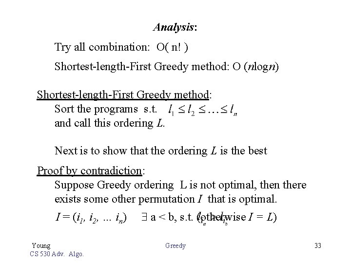
Analysis: Try all combination: O( n! ) Shortest-length-First Greedy method: O (nlogn) Shortest-length-First Greedy method: Sort the programs s. t. and call this ordering L. Next is to show that the ordering L is the best Proof by contradiction: Suppose Greedy ordering L is not optimal, then there exists some other permutation I that is optimal. I = (i 1, i 2, … in) a < b, s. t. (otherwise I = L) Young CS 530 Adv. Algo. Greedy 33

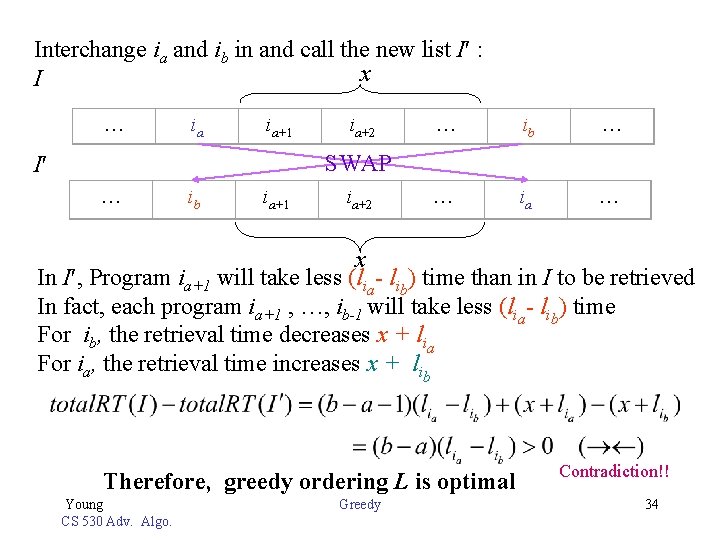
Interchange ia and ib in and call the new list I : x I … ia ia+1 ia+2 … ib … … ia … SWAP I … ib ia+1 ia+2 x In I , Program ia+1 will take less (lia- lib) time than in I to be retrieved In fact, each program ia+1 , …, ib-1 will take less (lia- lib) time For ib, the retrieval time decreases x + lia For ia, the retrieval time increases x + lib Therefore, greedy ordering L is optimal Young CS 530 Adv. Algo. Greedy Contradiction!! 34

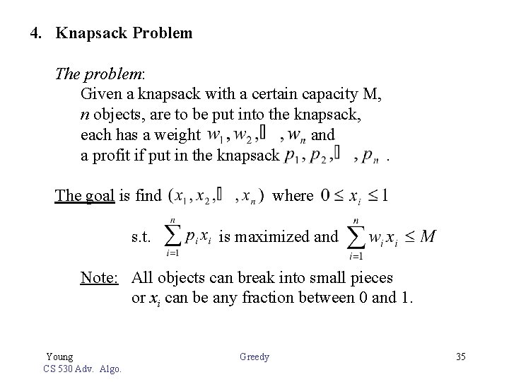
4. Knapsack Problem The problem: Given a knapsack with a certain capacity M, n objects, are to be put into the knapsack, each has a weight and a profit if put in the knapsack . The goal is find where s. t. is maximized and Note: All objects can break into small pieces or xi can be any fraction between 0 and 1. Young CS 530 Adv. Algo. Greedy 35

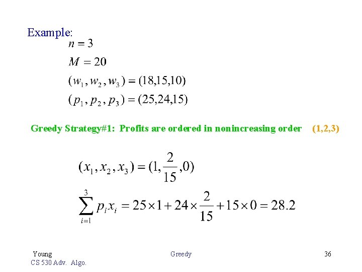
Example: Greedy Strategy#1: Profits are ordered in nonincreasing order (1, 2, 3) Young CS 530 Adv. Algo. Greedy 36

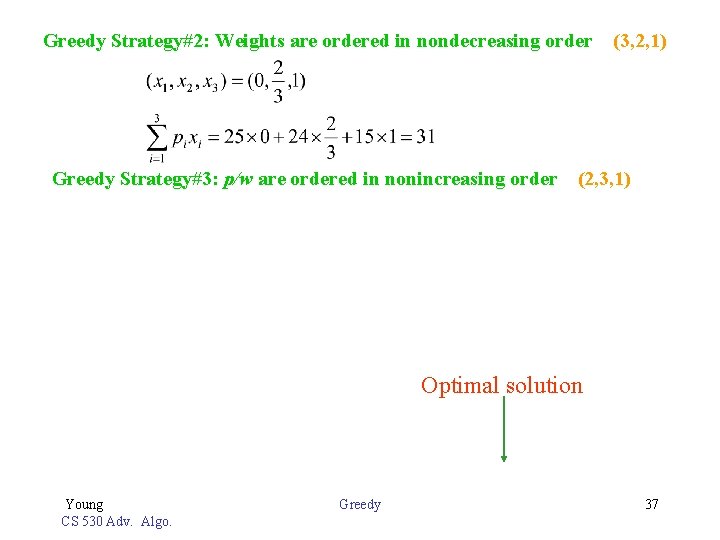
Greedy Strategy#2: Weights are ordered in nondecreasing order (3, 2, 1) Greedy Strategy#3: p/w are ordered in nonincreasing order (2, 3, 1) Optimal solution Young CS 530 Adv. Algo. Greedy 37

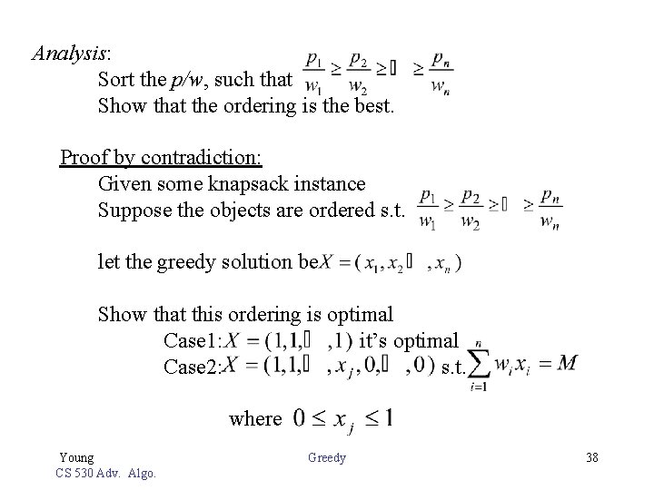
Analysis: Sort the p/w, such that Show that the ordering is the best. Proof by contradiction: Given some knapsack instance Suppose the objects are ordered s. t. let the greedy solution be Show that this ordering is optimal Case 1: it’s optimal Case 2: s. t. where Young CS 530 Adv. Algo. Greedy 38

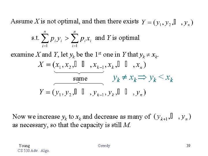
Assume X is not optimal, and then there exists s. t. and Y is optimal examine X and Y, let yk be the 1 st one in Y that yk xk yk < xk same Now we increase yk to xk and decrease as many of as necessary, so that the capacity is still M. Young CS 530 Adv. Algo. Greedy 39

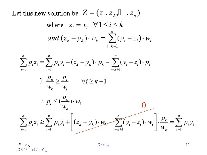
Let this new solution be where 0 Young CS 530 Adv. Algo. Greedy 40

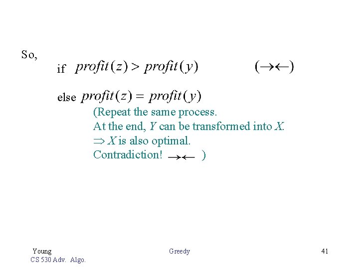
So, if else (Repeat the same process. At the end, Y can be transformed into X. X is also optimal. Contradiction! ) Young CS 530 Adv. Algo. Greedy 41