Supporting Aggregate Queries Over AdHoc Wireless Sensor Networks

Supporting Aggregate Queries Over Ad-Hoc Wireless Sensor Networks Samuel Madden UC Berkeley With Robert Szewczyk, Michael Franklin, and David Culler 1 WMCSA June 21, 2002

Motivation: Sensor Nets and In-Network Query Processing l l Many Sensor Network Applications are Data Oriented Queries Natural and Efficient Data Processing Mechanism – Easy (unlike embedded C code) Enable optimizations through abstraction – E. g. Which rooms are in use? – Sensor networks power and bandwidth constrained Communication dominates power cost Not subject to Moore’s law! – l l Aggregates Common Case In-network processing a must – – 2

Overview l Background – l Our Approach: Tiny Aggregation (TAG) – – – l 3 Sensor Networks Overview Expressiveness Illustration Optimizations Grouping Current Status & Future Work

Overview l Background – l Our Approach: Tiny Aggregation (TAG) – – – l 4 Sensor Networks Overview Expressiveness Illustration Optimizations Grouping Current Status & Future Work

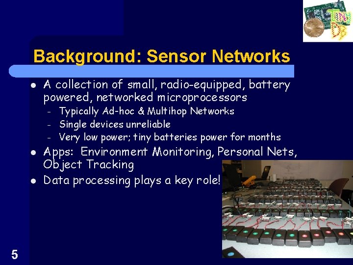
Background: Sensor Networks l A collection of small, radio-equipped, battery powered, networked microprocessors – – – l l 5 Typically Ad-hoc & Multihop Networks Single devices unreliable Very low power; tiny batteries power for months Apps: Environment Monitoring, Personal Nets, Object Tracking Data processing plays a key role!

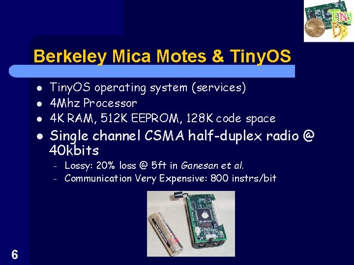
Berkeley Mica Motes & Tiny. OS l l Tiny. OS operating system (services) 4 Mhz Processor 4 K RAM, 512 K EEPROM, 128 K code space Single channel CSMA half-duplex radio @ 40 kbits – – 6 Lossy: 20% loss @ 5 ft in Ganesan et al. Communication Very Expensive: 800 instrs/bit

Overview l Background – l Our Approach: Tiny Aggregation (TAG) – – – l 7 Sensor Networks Overview Expressiveness Illustration Optimizations Grouping Current Status & Future Work

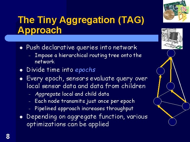
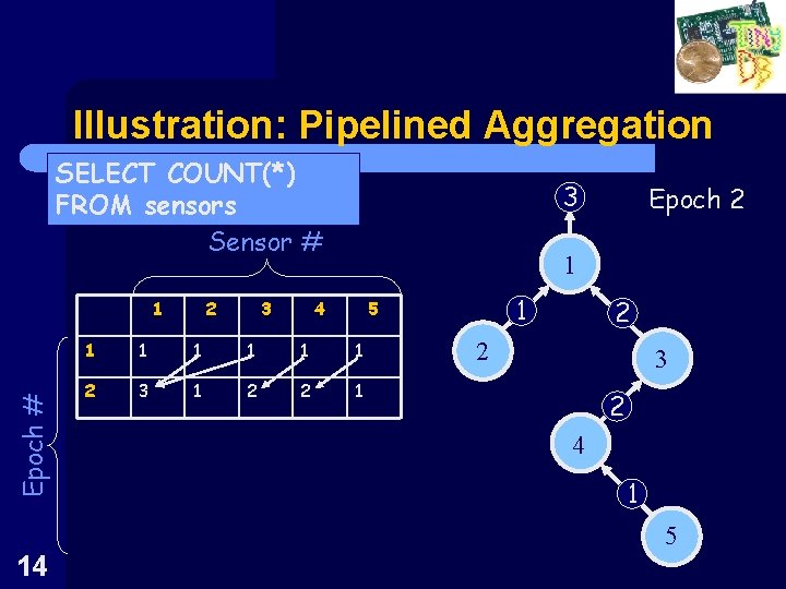
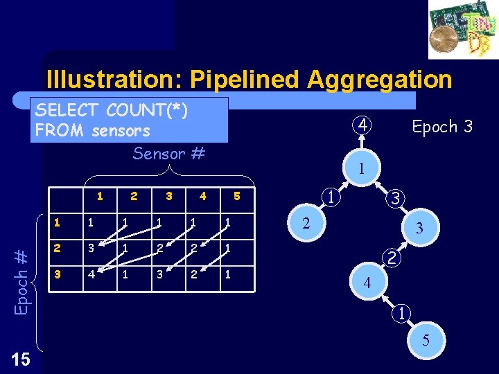
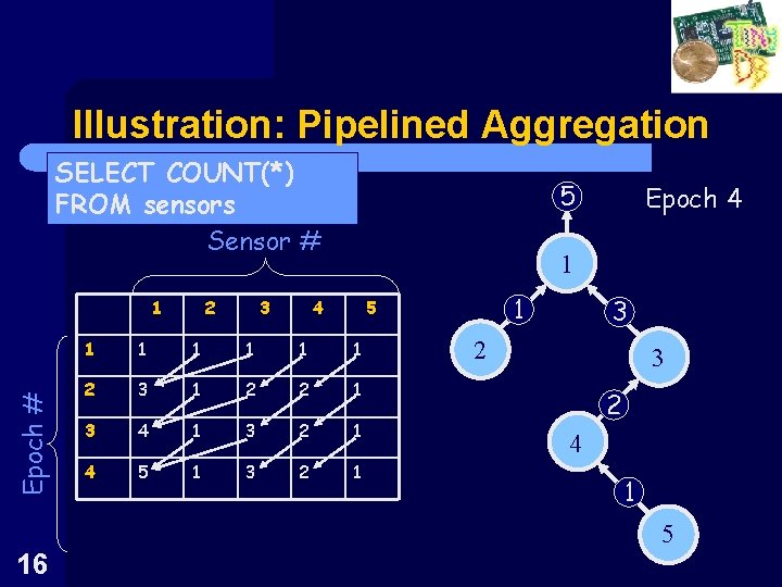
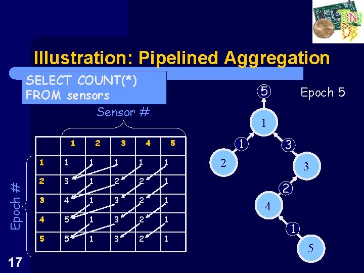
The Tiny Aggregation (TAG) Approach l Push declarative queries into network – l l Divide time into epochs Every epoch, sensors evaluate query over local sensor data and data from children – – – l 8 Impose a hierarchical routing tree onto the network Aggregate local and child data Each node transmits just once per epoch Pipelined approach increases throughput Depending on aggregate function, various optimizations can be applied

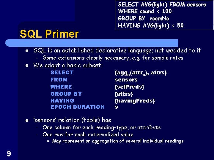
SQL Primer l SQL is an established declarative language; not wedded to it – l Some extensions clearly necessary, e. g. for sample rates We adopt a basic subset: SELECT FROM WHERE GROUP BY HAVING EPOCH DURATION l {aggn(attrn), attrs} sensors {sel. Preds} {attrs} {having. Preds} s ‘sensors’ relation (table) has – – One column for each reading-type, or attribute One row for each externalized value l 9 SELECT AVG(light) FROM sensors WHERE sound < 100 GROUP BY room. No HAVING AVG(light) < 50 May represent an aggregation of several individual readings

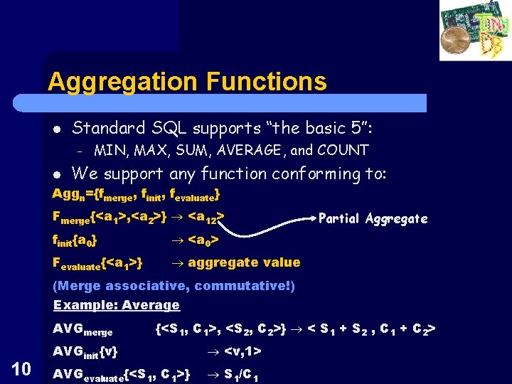
Aggregation Functions l Standard SQL supports “the basic 5”: – MIN, MAX, SUM, AVERAGE, and COUNT l We support any function Aggn={fmerge, finit, fevaluate} conforming to: Fmerge{<a 1>, <a 2>} <a 12> finit{a 0} <a 0> Fevaluate{<a 1>} aggregate value Partial Aggregate (Merge associative, commutative!) Example: Average AVGmerge 10 {<S 1, C 1>, <S 2, C 2>} < S 1 + S 2 , C 1 + C 2> AVGinit{v} <v, 1> AVGevaluate{<S 1, C 1>} S 1/C 1

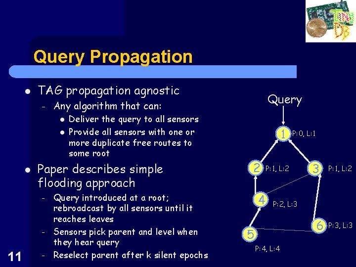
Query Propagation l TAG propagation agnostic – l l l – 11 Deliver the query to all sensors Provide all sensors with one or more duplicate free routes to some root Paper describes simple flooding approach – – Query Any algorithm that can: Query introduced at a root; rebroadcast by all sensors until it reaches leaves Sensors pick parent and level when they hear query Reselect parent after k silent epochs 1 2 4 P: 0, L: 1 P: 1, L: 2 3 P: 1, L: 2 P: 2, L: 3 6 5 P: 4, L: 4 P: 3, L: 3

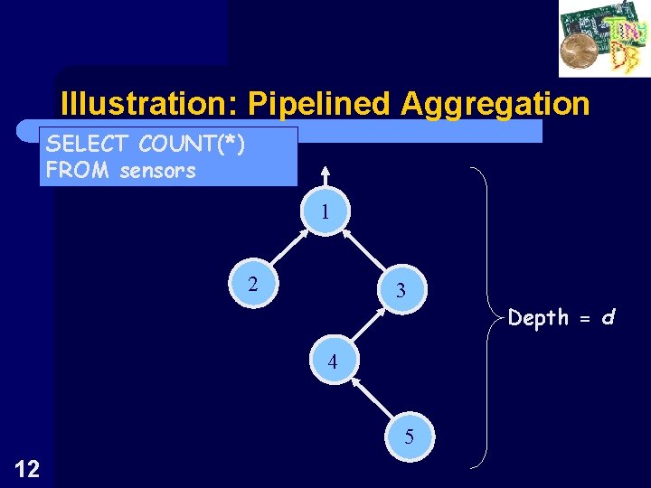
Illustration: Pipelined Aggregation SELECT COUNT(*) FROM sensors 1 2 3 4 5 12 Depth = d

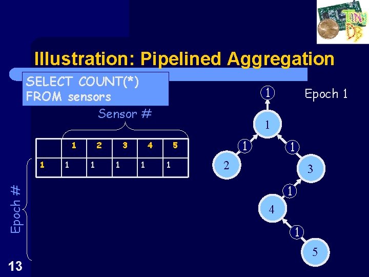
Illustration: Pipelined Aggregation SELECT COUNT(*) FROM sensors Sensor # 1 Epoch # 1 1 2 1 3 1 1 1 4 1 Epoch 1 1 5 1 1 2 3 1 4 1 5 13

Illustration: Pipelined Aggregation SELECT COUNT(*) FROM sensors Sensor # Epoch # 1 2 3 3 Epoch 2 1 4 1 5 1 1 1 2 3 1 2 2 3 2 4 1 5 14

Illustration: Pipelined Aggregation SELECT COUNT(*) FROM sensors Sensor # Epoch # 1 2 3 4 Epoch 3 1 4 1 5 1 1 1 2 3 1 2 2 1 3 4 1 3 2 3 2 4 1 5 15

Illustration: Pipelined Aggregation SELECT COUNT(*) FROM sensors Sensor # Epoch # 1 2 3 5 Epoch 4 1 5 1 1 1 2 3 1 2 2 1 3 4 1 3 2 1 4 5 1 3 2 3 2 4 1 5 16

Illustration: Pipelined Aggregation SELECT COUNT(*) FROM sensors Sensor # Epoch # 1 17 2 3 5 Epoch 5 1 4 1 5 1 1 1 2 3 1 2 2 1 3 4 1 3 2 1 4 5 1 3 2 1 5 5 1 3 2 3 2 4 1 5

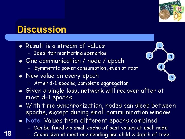
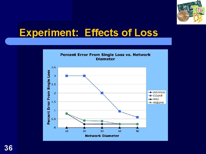
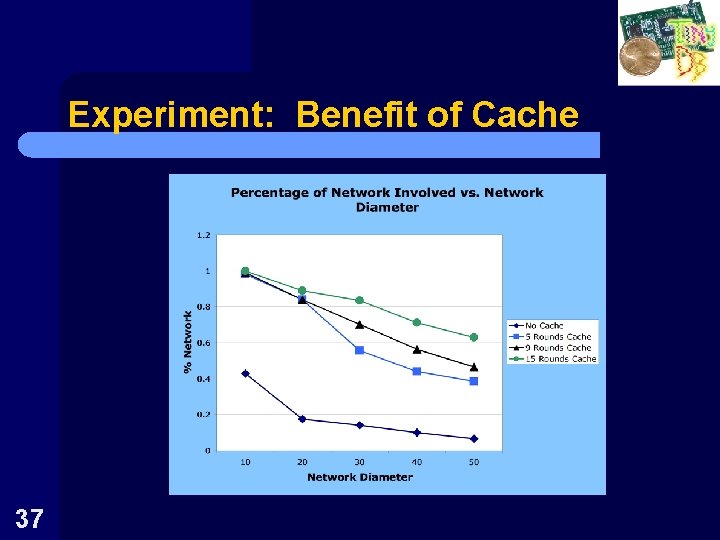
Discussion l l l 18 Result is a stream of values – Ideal for monitoring scenarios – Symmetric power consumption, even at root One communication / node / epoch 1 2 3 4 New value on every epoch – After d-1 epochs, complete aggregation – Can be fixed via small cache of past values at each node Cache size at most one reading per child x depth of tree 5 Given a single loss, network will recover after at most d-1 epochs With time synchronization, nodes can sleep between epochs, except during small communication window Note: Values from different epochs combined –

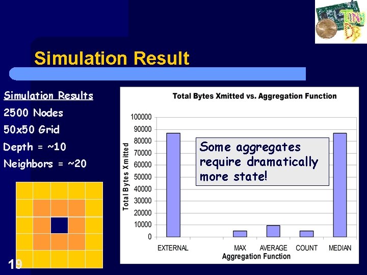
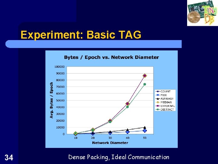
Simulation Results 2500 Nodes 50 x 50 Grid Depth = ~10 Neighbors = ~20 19 Some aggregates require dramatically more state!

Optimization: Channel Sharing l l Insight: Shared channel enables optimizations Suppress messages that won’t affect aggregate – – l E. g. , in a MAX query, sensor with value v hears a neighbor with value ≥ v, so it doesn’t report Applies to all such exemplary aggregates Learn about query advertisements it missed – If a sensor shows up in a new environment, it can learn about queries by looking at neighbors messages. l 20 Root doesn’t have to explicitly rebroadcast query!

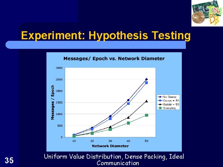
Optimization: Hypothesis Testing l Insight: Root can provide information that will suppress readings that cannot affect the final aggregate value. – – l How is hypothesis computed? – – – 21 E. g. Tell all the nodes that the MIN is definitely < 50; nodes with value ≥ 50 need not participate. Works for any linear aggregate function Blind guess Statistically informed guess Observation over first few levels of tree / rounds of aggregate

Optimization: Use Multiple Parents l For duplicate insensitive (e. g. MAX), or partitionable (e. g. COUNT) aggregates, – – Send (part of) aggregate to all parents Decreases variance l l 22 Dramatically, when there are lots of parents No extra cost, since all messages broadcast

Grouping l l Value-based, complete partitioning of records If query is grouped, sensors apply predicate to local readings on each epoch Aggregate records tagged with group When a child record (with group) is received: – – l l At the end of each epoch, transmit one record per group Number of groups may exceed available storage – 23 If it belongs to a stored group, merge with existing record for that group If not, just store it Can evict groups for aggregation at root!

Overview l Background – l Our Approach: Tiny Aggregation (TAG) – – – l 24 Sensor Networks Overview Expressiveness Illustration Optimizations Grouping Current Status & Future Work

Status & Future Work l Status – Simple simulator l – Generalization of algorithms beyond complete pipelining Taxonomy of aggregates to allow optimizations on functional properties Basic implementation (shown in demo) – Expressiveness issues – – l Future work l l – 25 Complete set of experiments, including behavior of algorithms in the face of loss Aggregates over temporal data Nested queries, e. g MAX(AVG(1000 readings) @ each node) Correctness Issues in The Face Of Loss l How does the user know which nodes are and are not included in an aggregate?

Summary l Declarative queries for aggregates – – Straightforward, familiar interface Enables optimizations l l l Pipelined, epoch based algorithm – – – 26 Snooping techniques for exemplary aggregates Multiple parents for partitionable aggregates Streaming Results Symmetric communication Low-power friendly

Questions? 27

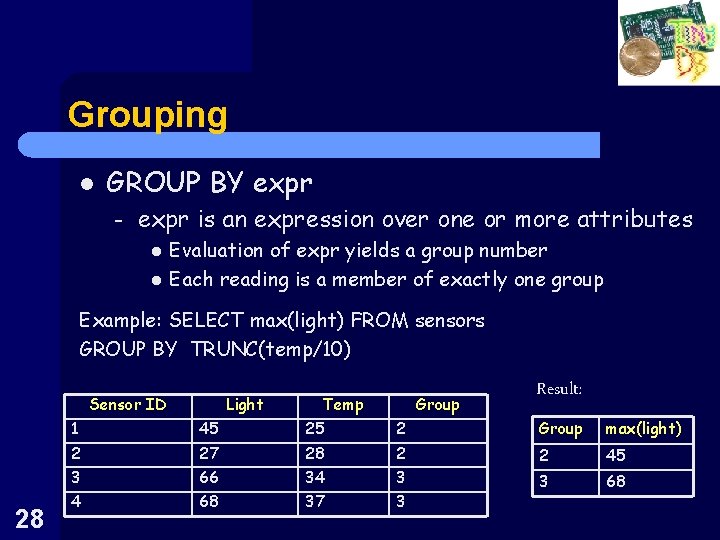
Grouping l GROUP BY expr – expr is an expression over one or more attributes l l Evaluation of expr yields a group number Each reading is a member of exactly one group Example: SELECT max(light) FROM sensors GROUP BY TRUNC(temp/10) Sensor ID 28 Light Temp Group Result: 1 45 25 2 Group max(light) 2 27 28 2 3 66 34 3 2 45 4 68 37 3 3 68

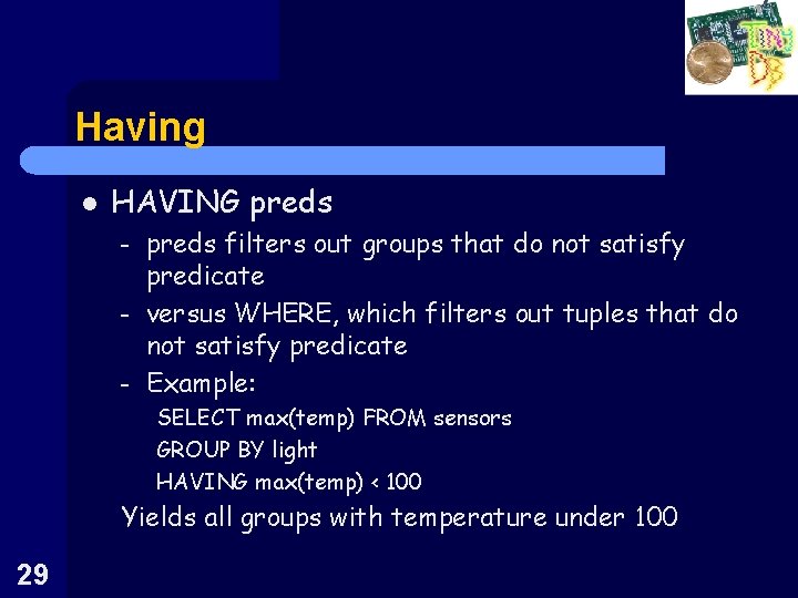
Having l HAVING preds – – – preds filters out groups that do not satisfy predicate versus WHERE, which filters out tuples that do not satisfy predicate Example: SELECT max(temp) FROM sensors GROUP BY light HAVING max(temp) < 100 Yields all groups with temperature under 100 29

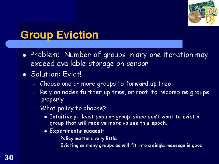
Group Eviction l l Problem: Number of groups in any one iteration may exceed available storage on sensor Solution: Evict! – – – Choose one or more groups to forward up tree Rely on nodes further up tree, or root, to recombine groups properly What policy to choose? l l Intuitively: least popular group, since don’t want to evict a group that will receive more values this epoch. Experiments suggest: Policy matters very little – Evicting as many groups as will fit into a single message is good – 30

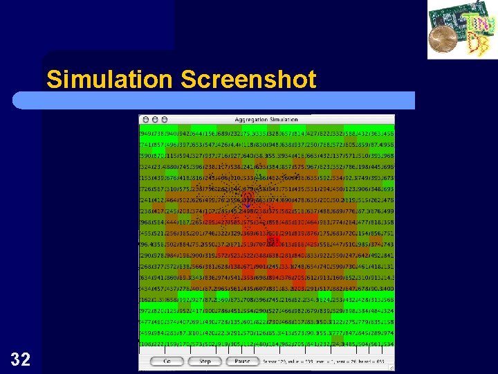
Simulation Environment l l Java-based simulation & visualization for validating algorithms, collecting data. Coarse grained event based simulation – – Sensors arranged on a grid, radio connectivity by Euclidian distance Communication model l l 31 Lossless: All neighbors hear all messages Lossy: Messages lost with probability that increases with distance Symmetric links No collisions, hidden terminals, etc.

Simulation Screenshot 32

Experimental Results l Experiments with simulator – – – l Most experiments in terms of bytes or messages sent, since message transmission is the dominant cost – 33 Performance of basic TAG Benefits of hypothesis testing Effect of loss Depends on radio being turned off between epochs and aggregation functions being cheap

Experiment: Basic TAG 34 Dense Packing, Ideal Communication

Experiment: Hypothesis Testing 35 Uniform Value Distribution, Dense Packing, Ideal Communication

Experiment: Effects of Loss 36

Experiment: Benefit of Cache 37

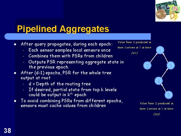
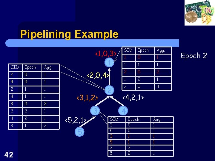
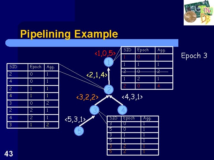
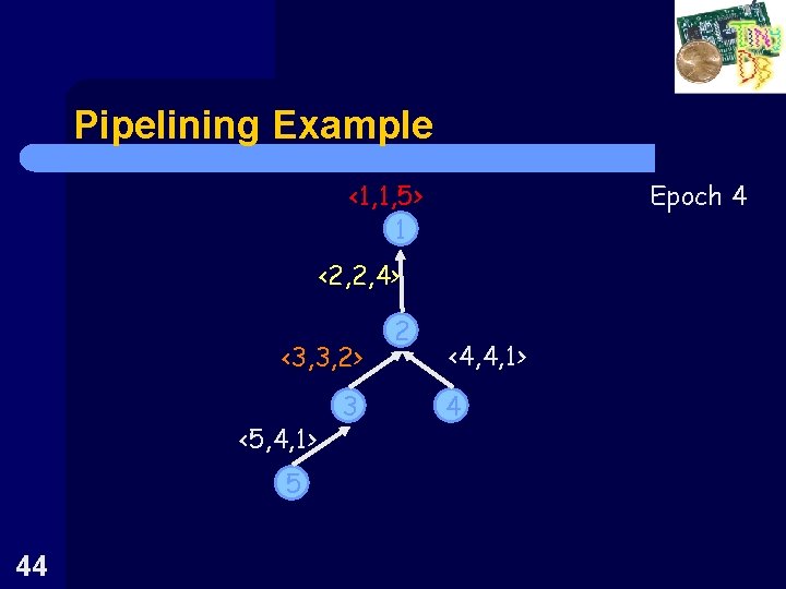
Pipelined Aggregates l l l Value from 2 produced at After query propagates, during each epoch: time t arrives at 1 at time – Each sensor samples local sensors once 1 (t+1) – Combines them with PSRs from children – Outputs PSR representing aggregate state in 3 2 the previous epoch. After (d-1) epochs, PSR for the whole tree output at root 4 – d = Depth of the routing tree – If desired, partial state from top k levels could be output in kth epoch 5 To avoid combining PSRs from different epochs, Value from 5 produced at sensors must cache values from children time t arrives at 1 at time (t+3) 38

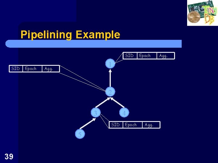
Pipelining Example SID Epoch 1 Agg. 2 3 4 SID 5 39 Epoch Agg.

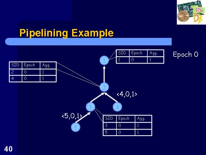
Pipelining Example SID Epoch Agg. 2 0 1 4 0 1 1 2 <5, 0, 1> 5 40 3 SID Epoch Agg. 1 0 1 <4, 0, 1> 4 SID Epoch Agg. 3 0 1 5 0 1 Epoch 0

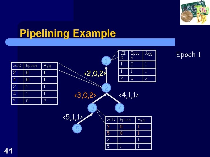
Pipelining Example SID Epoch Agg. 2 0 1 4 0 1 2 1 1 4 1 1 3 0 2 1 <2, 0, 2> <3, 0, 2> <5, 1, 1> 5 41 2 3 SI D Epoc h Agg. 1 0 1 1 2 0 2 <4, 1, 1> 4 SID Epoch Agg. 3 0 1 5 0 1 3 1 1 5 1 1 Epoch 1

Pipelining Example SID Epoch Agg. 2 0 1 4 0 1 2 1 1 4 1 1 3 0 2 2 2 1 4 2 1 3 1 2 42 <1, 0, 3> 1 <2, 0, 4> <3, 1, 2> <5, 2, 1> 5 2 3 SID Epoch Agg. 1 0 1 1 2 0 2 1 2 0 4 <4, 2, 1> 4 SID 3 5 3 5 Epoch 0 0 1 1 2 2 Agg. 1 1 1 Epoch 2

Pipelining Example SID Epoch Agg. 2 0 1 4 0 1 2 1 1 4 1 1 3 0 2 2 2 1 4 2 1 3 1 2 43 <1, 0, 5> 1 <2, 1, 4> <3, 2, 2> <5, 3, 1> 5 3 2 SID 3 5 3 5 SID Epoch Agg. 1 0 1 1 2 0 2 1 2 0 4 <4, 3, 1> 4 Epoch 0 0 1 1 2 2 Agg. 1 1 1 Epoch 3

Pipelining Example Epoch 4 <1, 1, 5> 1 <2, 2, 4> <3, 3, 2> <5, 4, 1> 5 44 3 2 <4, 4, 1> 4

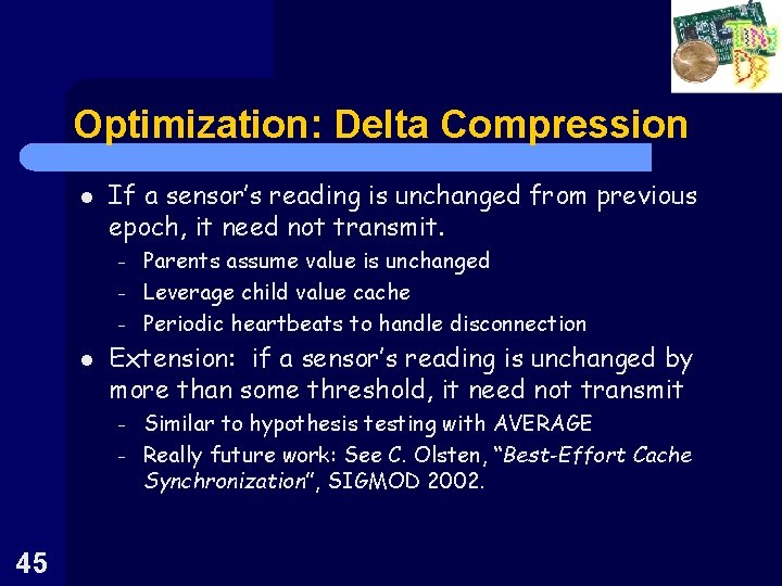
Optimization: Delta Compression l If a sensor’s reading is unchanged from previous epoch, it need not transmit. – – – l Extension: if a sensor’s reading is unchanged by more than some threshold, it need not transmit – – 45 Parents assume value is unchanged Leverage child value cache Periodic heartbeats to handle disconnection Similar to hypothesis testing with AVERAGE Really future work: See C. Olsten, “Best-Effort Cache Synchronization”, SIGMOD 2002.

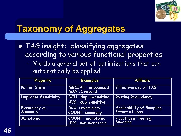
Taxonomy of Aggregates l TAG insight: classifying aggregates according to various functional properties – Yields a general set of optimizations that can automatically be applied Property Partial State Duplicate Sensitivity Exemplary vs. Summary Monotonic 46 Examples MEDIAN : unbounded, MAX : 1 record MIN : dup. insensitive, AVG : dup. sensitive MAX : exemplary COUNT: summary COUNT : monotonic AVG : non-monotonic Affects Effectiveness of TAG Routing Redundancy Applicability of Sampling, Effect of Loss Hypothesis Testing, Snooping

47