Sensor Selection in AdHoc Wireless Sensor Networks Olawoye

Sensor Selection in Ad-Hoc Wireless Sensor Networks Olawoye Oyeyele 10/10/2003

Outline l l Sensor Selection Problem Randomization Spatial Selection Discussions

Sensor Selection Problem l l l Densely deployed wireless sensor networks consume energy through communications Not all measured data necessarily required for detection Subset of data may provide acceptable detection

Objectives l l l Robust selection Acceptable performance Minimum complexity

Randomization[3] l l l Algorithm divides data from sensors into time slots. In every time slot each sensor in the cluster randomly determines whether or not to transmit its measurement to the base station The probability of selection is a small value

Possible Demerits l l May result in a biased selection of data – data may be taken from one corner of the network Data may not be representative of the entire network Puts a lot of burden on the manager node (cluster head/base station). Differences in number of selected sensors per trial leads to variations in detector performance.

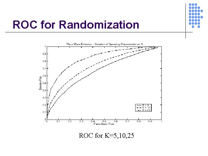
ROC for Randomization ROC for K=5, 10, 25

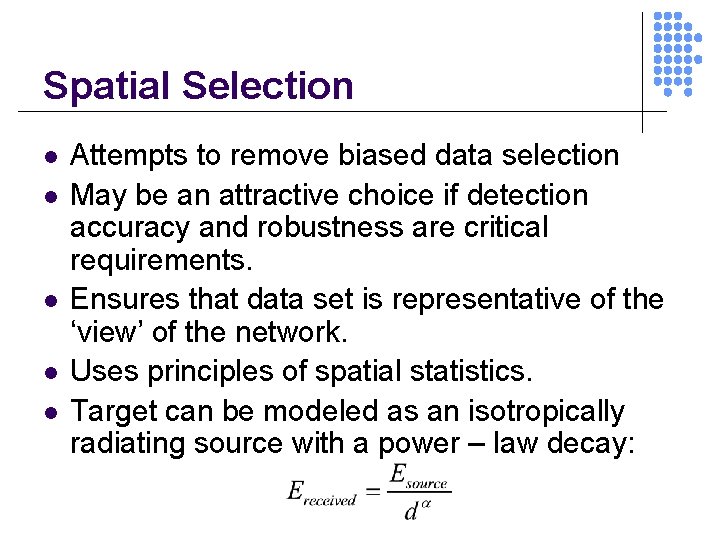
Spatial Selection l l l Attempts to remove biased data selection May be an attractive choice if detection accuracy and robustness are critical requirements. Ensures that data set is representative of the ‘view’ of the network. Uses principles of spatial statistics. Target can be modeled as an isotropically radiating source with a power – law decay:

Spatial Statistics l l l Applying statistical methods to data that are spatially distributed Techniques used extensively in geostatistics and GIS Major component is spatial dependence l l Spatial dependence based on the fact that data in a small section of space can be similar hence redundant i. e. little additional information provided) The Variogram is the major tool used in estimating spatial dependence.

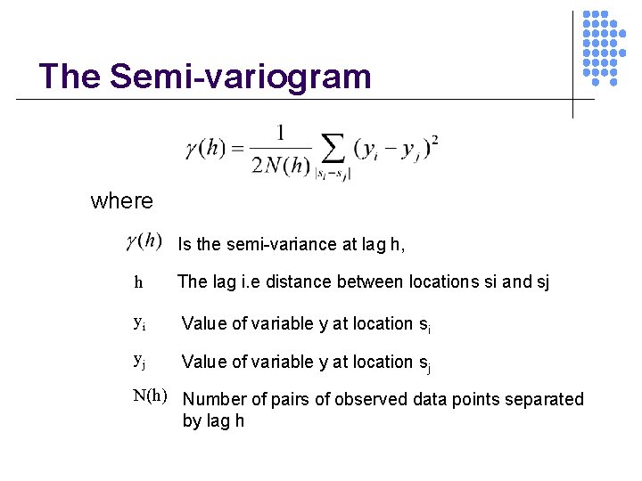
The Semi-variogram where Is the semi-variance at lag h, h The lag i. e distance between locations si and sj yi Value of variable y at location si yj Value of variable y at location sj N(h) Number of pairs of observed data points separated by lag h

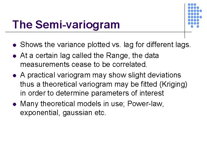
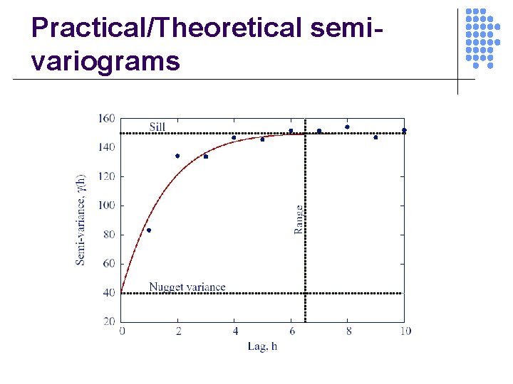
The Semi-variogram l l Shows the variance plotted vs. lag for different lags. At a certain lag called the Range, the data measurements cease to be correlated. A practical variogram may show slight deviations thus a theoretical variogram may be fitted (Kriging) in order to determine parameters of interest Many theoretical models in use; Power-law, exponential, gaussian etc.

Practical/Theoretical semivariograms

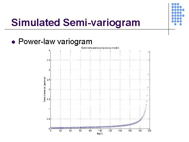
Simulated Semi-variogram l Power-law variogram

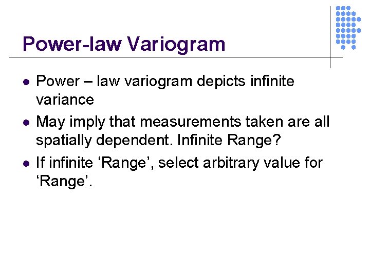
Power-law Variogram l l l Power – law variogram depicts infinite variance May imply that measurements taken are all spatially dependent. Infinite Range? If infinite ‘Range’, select arbitrary value for ‘Range’.

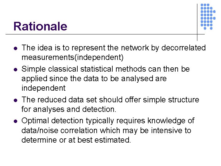
Rationale l l The idea is to represent the network by decorrelated measurements(independent) Simple classical statistical methods can then be applied since the data to be analysed are independent The reduced data set should offer simple structure for analyses and detection. Optimal detection typically requires knowledge of data/noise correlation which may be intensive to determine or at best estimated.

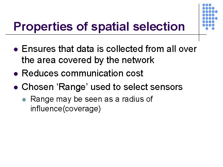
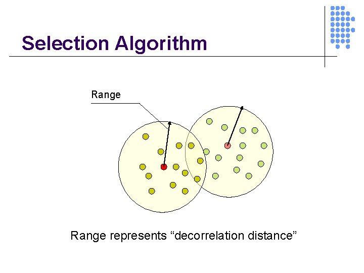
Properties of spatial selection l l l Ensures that data is collected from all over the area covered by the network Reduces communication cost Chosen ‘Range’ used to select sensors l Range may be seen as a radius of influence(coverage)

Selection Algorithm Range represents “decorrelation distance”

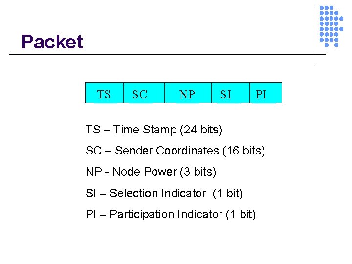
Packet TS SC NP SI PI TS – Time Stamp (24 bits) SC – Sender Coordinates (16 bits) NP - Node Power (3 bits) SI – Selection Indicator (1 bit) PI – Participation Indicator (1 bit)

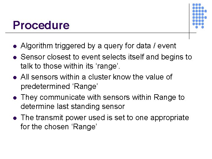
Procedure l l l Algorithm triggered by a query for data / event Sensor closest to event selects itself and begins to talk to those within its ‘range’. All sensors within a cluster know the value of predetermined ‘Range’ They communicate with sensors within Range to determine last standing sensor The transmit power used is set to one appropriate for the chosen ‘Range’

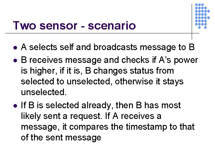
Two sensor - scenario l l l A selects self and broadcasts message to B B receives message and checks if A’s power is higher, if it is, B changes status from selected to unselected, otherwise it stays unselected. If B is selected already, then B has most likely sent a request. If A receives a message, it compares the timestamp to that of the sent message

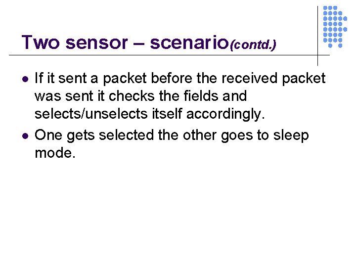
Two sensor – scenario(contd. ) l l If it sent a packet before the received packet was sent it checks the fields and selects/unselects itself accordingly. One gets selected the other goes to sleep mode.

Simulation Directions l l l Detector Performance (Receiver Operating Characteristic) Energy consumption Theoretical characteristics of the detector. l l Randomization leads to complex detector properties that are only implementable through approximations Demonstrate that chosen subset achieves coverage[4]

Discussions l Spatial Selection promises to be a robust selection technique l l l Consistent, stable performance Complexity may be further reduced if combined with a reactive clustering technique such as De. Re. Clus Increased network lifetime

References 1. 2. 3. 4. 5. Clark Isobel, ‘Practical Geostatistics’ (on the web) Xu Yingyue, Hairong Qi, ’Decentralized Reactive Clustering in Collaborative Processing Using Different Computing Paradigms’ Sestok C. K. , Maya R. Said, Alan V. Oppenheim, ’Randomized Data Selection in Detection with Applications to Distributed Signal Processing’, Proceedings of the IEEE, September, 2003 Dalenius T. , Jaroslav Hajek, Stefan Zubrzycki, ’On plane sampling and Related Geometrical Problems’, Fourth Berkeley Symposium, 1961. Ripley Brian D. , ’Spatial Statistics’, John Wiley and Sons, 1981.

Advances in Energy Research l Two new advances in energy l l Fuel cell ( Motor cars, laptops etc) – still large form factor , research is active Power paper - Thin and likely to revolutionize miniaturization