Supply and Demand n The Supply Curve l

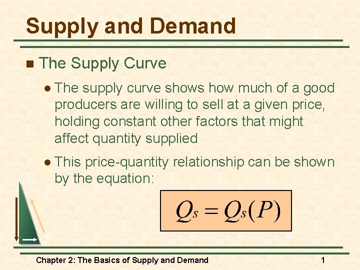
Supply and Demand n The Supply Curve l The supply curve shows how much of a good producers are willing to sell at a given price, holding constant other factors that might affect quantity supplied l This price-quantity relationship can be shown by the equation: Chapter 2: The Basics of Supply and Demand 1

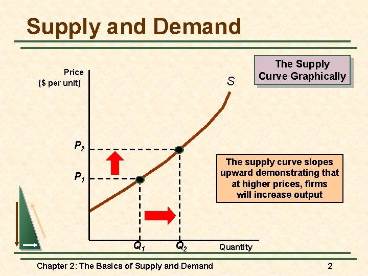
Supply and Demand Price ($ per unit) S The Supply Curve Graphically P 2 The supply curve slopes upward demonstrating that at higher prices, firms will increase output P 1 Q 2 Chapter 2: The Basics of Supply and Demand Quantity 2

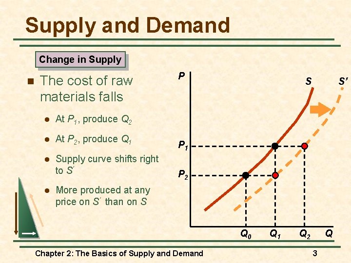
Supply and Demand Change in Supply n The cost of raw materials falls l At P 1, produce Q 2 l At P 2, produce Q 1 l Supply curve shifts right to S’ l P S S’ P 1 P 2 More produced at any price on S’ than on S Q 0 Chapter 2: The Basics of Supply and Demand Q 1 Q 2 Q 3

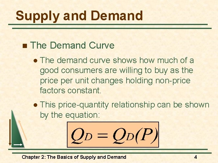
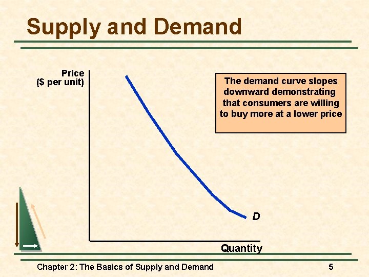
Supply and Demand n The Demand Curve l The demand curve shows how much of a good consumers are willing to buy as the price per unit changes holding non-price factors constant. l This price-quantity relationship can be shown by the equation: Chapter 2: The Basics of Supply and Demand 4

Supply and Demand Price ($ per unit) The demand curve slopes downward demonstrating that consumers are willing to buy more at a lower price D Quantity Chapter 2: The Basics of Supply and Demand 5

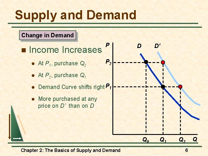
Supply and Demand Change in Demand n Income Increases P D D’ P 2 l At P 1, purchase Q 2 l At P 2, purchase Q 1 l Demand Curve shifts right P 1 l More purchased at any price on D’ than on D Q 0 Chapter 2: The Basics of Supply and Demand Q 1 Q Q 2 6

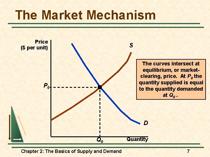
The Market Mechanism Price ($ per unit) S The curves intersect at equilibrium, or marketclearing, price. At P 0 the quantity supplied is equal to the quantity demanded at Q 0. P 0 D Q 0 Chapter 2: The Basics of Supply and Demand Quantity 7

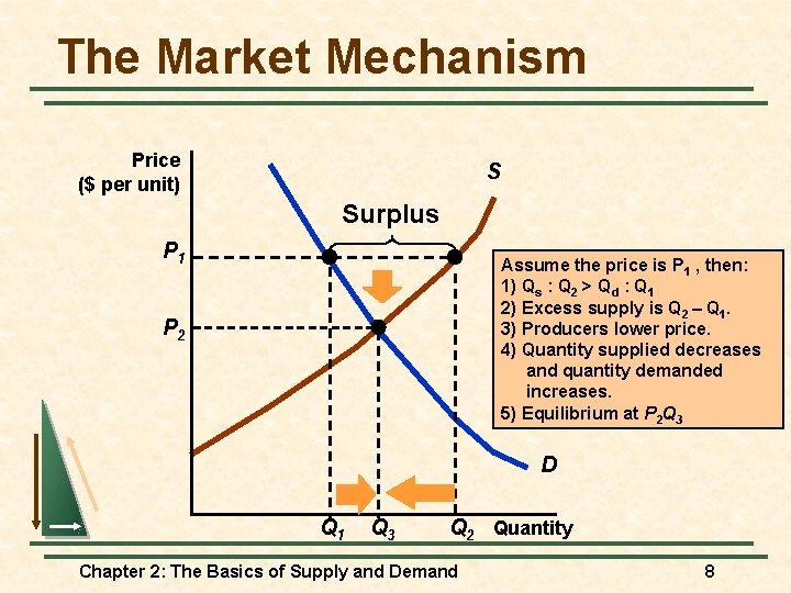
The Market Mechanism Price ($ per unit) S Surplus P 1 Assume the price is P 1 , then: 1) Qs : Q 2 > Qd : Q 1 2) Excess supply is Q 2 – Q 1. 3) Producers lower price. 4) Quantity supplied decreases and quantity demanded increases. 5) Equilibrium at P 2 Q 3 P 2 D Q 1 Q 3 Q 2 Quantity Chapter 2: The Basics of Supply and Demand 8

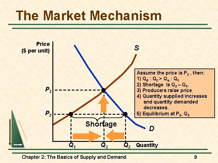
The Market Mechanism Price ($ per unit) S Assume the price is P 2 , then: 1) Qd : Q 2 > Qs : Q 1 2) Shortage is Q 2 – Q 1. 3) Producers raise price. 4) Quantity supplied increases and quantity demanded decreases. 5) Equilibrium at P 3, Q 3 P 2 Shortage Q 1 Q 3 D Q 2 Quantity Chapter 2: The Basics of Supply and Demand 9

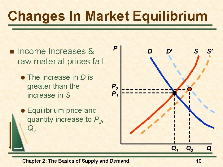
Changes In Market Equilibrium n Income Increases & raw material prices fall l l The increase in D is greater than the increase in S P D D’ S S’ P 2 P 1 Equilibrium price and quantity increase to P 2, Q 2 Q 1 Chapter 2: The Basics of Supply and Demand Q 2 Q 10

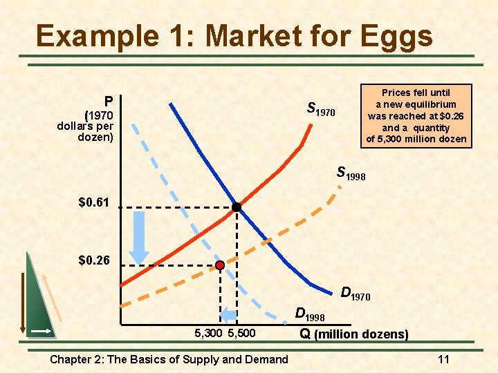
Example 1: Market for Eggs P Prices fell until a new equilibrium was reached at $0. 26 and a quantity of 5, 300 million dozen S 1970 (1970 dollars per dozen) S 1998 $0. 61 $0. 26 D 1970 5, 300 5, 500 Chapter 2: The Basics of Supply and Demand D 1998 Q (million dozens) 11

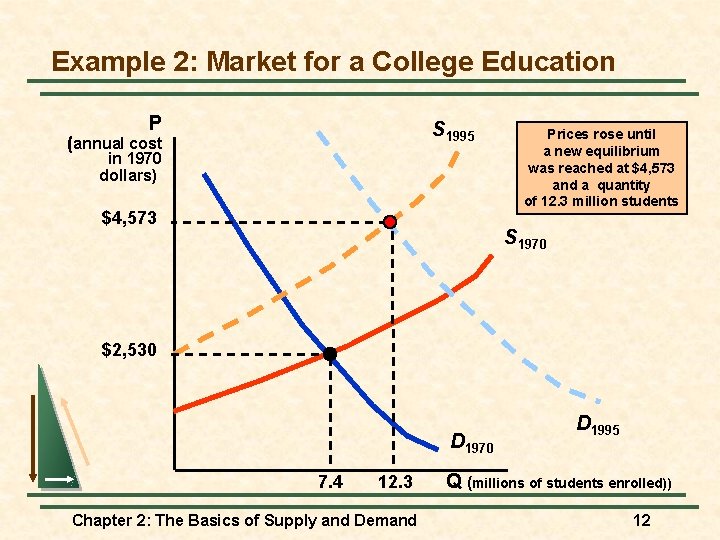
Example 2: Market for a College Education P S 1995 (annual cost in 1970 dollars) $4, 573 Prices rose until a new equilibrium was reached at $4, 573 and a quantity of 12. 3 million students S 1970 $2, 530 D 1970 7. 4 12. 3 Chapter 2: The Basics of Supply and Demand D 1995 Q (millions of students enrolled)) 12

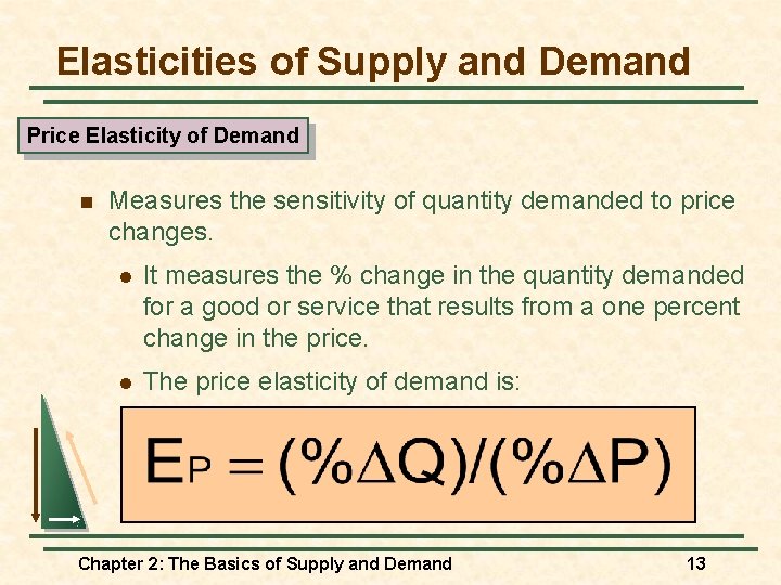
Elasticities of Supply and Demand Price Elasticity of Demand n Measures the sensitivity of quantity demanded to price changes. l It measures the % change in the quantity demanded for a good or service that results from a one percent change in the price. l The price elasticity of demand is: Chapter 2: The Basics of Supply and Demand 13

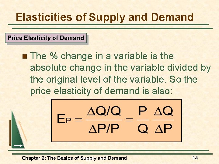
Elasticities of Supply and Demand Price Elasticity of Demand n The % change in a variable is the absolute change in the variable divided by the original level of the variable. So the price elasticity of demand is also: Chapter 2: The Basics of Supply and Demand 14

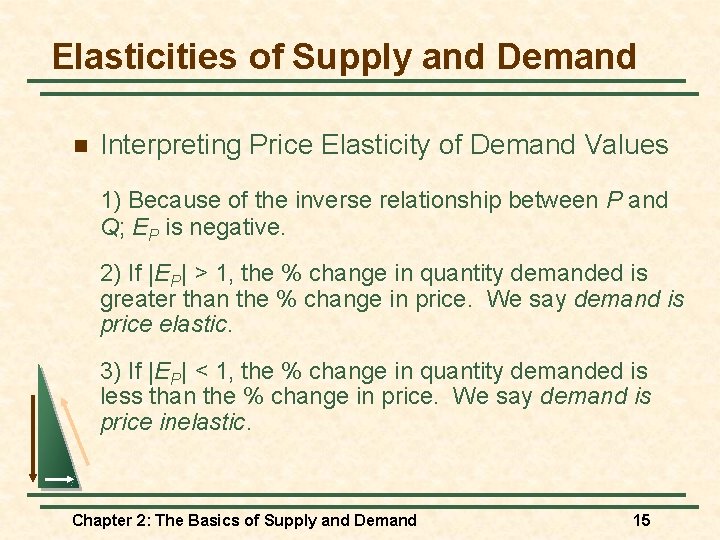
Elasticities of Supply and Demand n Interpreting Price Elasticity of Demand Values 1) Because of the inverse relationship between P and Q; EP is negative. 2) If |EP| > 1, the % change in quantity demanded is greater than the % change in price. We say demand is price elastic. 3) If |EP| < 1, the % change in quantity demanded is less than the % change in price. We say demand is price inelastic. Chapter 2: The Basics of Supply and Demand 15

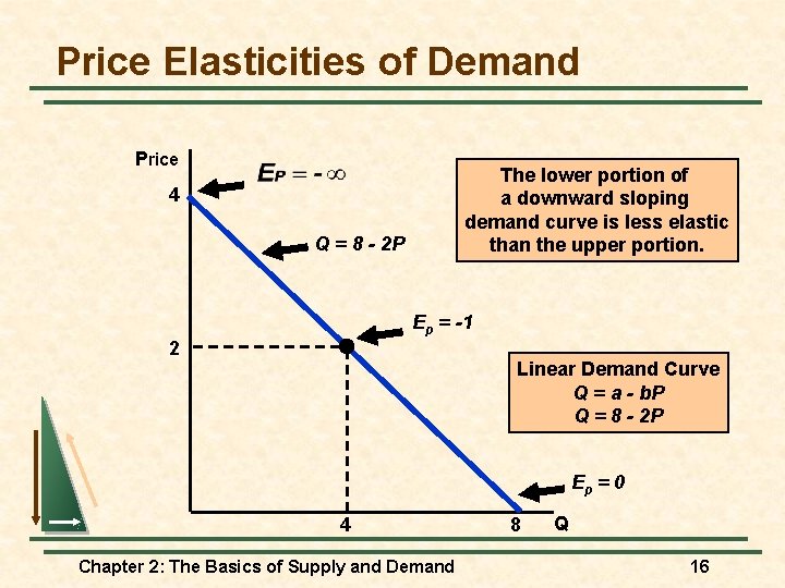
Price Elasticities of Demand Price The lower portion of a downward sloping demand curve is less elastic than the upper portion. 4 Q = 8 - 2 P Ep = -1 2 Linear Demand Curve Q = a - b. P Q = 8 - 2 P Ep = 0 4 Chapter 2: The Basics of Supply and Demand 8 Q 16

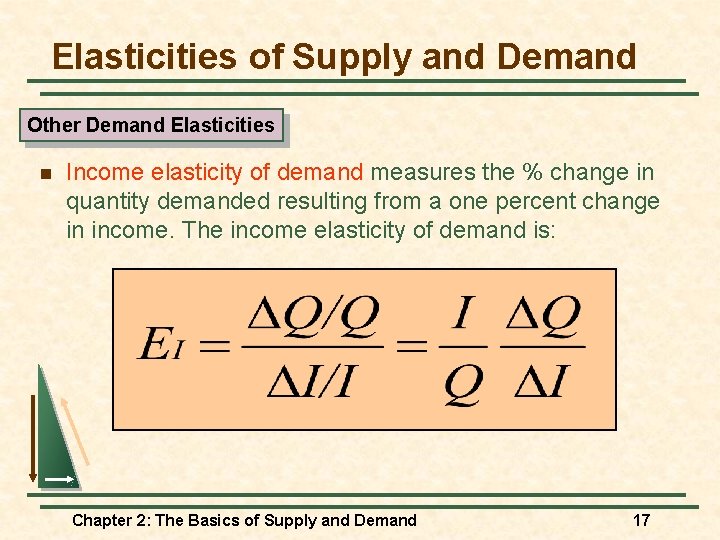
Elasticities of Supply and Demand Other Demand Elasticities n Income elasticity of demand measures the % change in quantity demanded resulting from a one percent change in income. The income elasticity of demand is: Chapter 2: The Basics of Supply and Demand 17

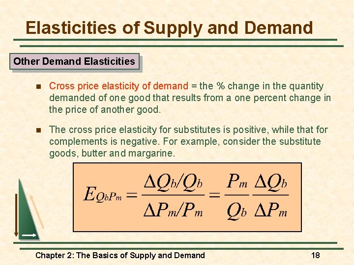
Elasticities of Supply and Demand Other Demand Elasticities n Cross price elasticity of demand = the % change in the quantity demanded of one good that results from a one percent change in the price of another good. n The cross price elasticity for substitutes is positive, while that for complements is negative. For example, consider the substitute goods, butter and margarine. Chapter 2: The Basics of Supply and Demand 18

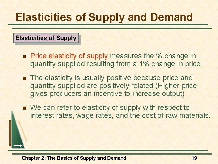
Elasticities of Supply and Demand Elasticities of Supply n Price elasticity of supply measures the % change in quantity supplied resulting from a 1% change in price. n The elasticity is usually positive because price and quantity supplied are positively related (Higher price gives producers an incentive to increase output) n We can refer to elasticity of supply with respect to interest rates, wage rates, and the cost of raw materials. Chapter 2: The Basics of Supply and Demand 19

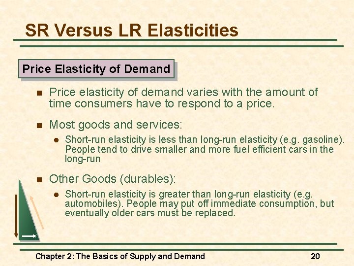
SR Versus LR Elasticities Price Elasticity of Demand n Price elasticity of demand varies with the amount of time consumers have to respond to a price. n Most goods and services: l n Short-run elasticity is less than long-run elasticity (e. g. gasoline). People tend to drive smaller and more fuel efficient cars in the long-run Other Goods (durables): l Short-run elasticity is greater than long-run elasticity (e. g. automobiles). People may put off immediate consumption, but eventually older cars must be replaced. Chapter 2: The Basics of Supply and Demand 20

SR Versus LR Elasticities Income Elasticities n Most goods and services: l Income elasticity is greater in the long-run than in the short run. For example, higher incomes may be converted into bigger cars so the income elasticity of demand for gasoline increases with time. n Other Goods (durables): l Income elasticity is less in the long-run than in the short-run. For example, consumers will initially want to hold more cars. Later, purchases will only to be to replace old cars. Chapter 2: The Basics of Supply and Demand 21

SR Versus LR Elasticities Price Elasticity of Supply n Most goods and services: l n Long-run price elasticity of supply is greater than short-run price elasticity of supply. Due to limited capacity, firms are output constrained in the short-run. In the long-run, they can expand. Other Goods (durables, recyclables): l Long-run price elasticity of supply is less than short-run price elasticity of supply. For example, consider the secondary copper market. Copper price increases provide an incentive to convert scrap copper into new supply. In the long-run, this stock of scrap copper begins to fall. Chapter 2: The Basics of Supply and Demand 22

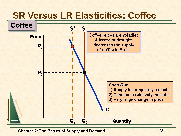
SR Versus LR Elasticities: Coffee S’ S Coffee prices are volatile: A freeze or drought decreases the supply of coffee in Brazil Price P 1 P 0 Short-Run 1) Supply is completely inelastic 2) Demand is relatively inelastic 3) Very large change in price D Q 1 Q 0 Chapter 2: The Basics of Supply and Demand Quantity 23

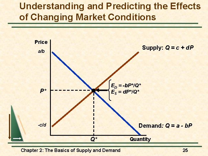
Understanding and Predicting the Effects of Changing Market Conditions 1. We must learn how to “fit” linear demand supply curves to market data. 2. We determine numerically how a change in one variable will cause supply or demand to shift and so affect the equilibrium price and quantity. 3. Assume the Available Data are: l Equilibrium Price, P* l Equilibrium Quantity, Q* l Price elasticity of supply, ES, and demand, ED. Chapter 2: The Basics of Supply and Demand 24

Understanding and Predicting the Effects of Changing Market Conditions Price Supply: Q = c + d. P a/b ED = -b. P*/Q* ES = d. P*/Q* P* -c/d Demand: Q = a - b. P Q* Chapter 2: The Basics of Supply and Demand Quantity 25

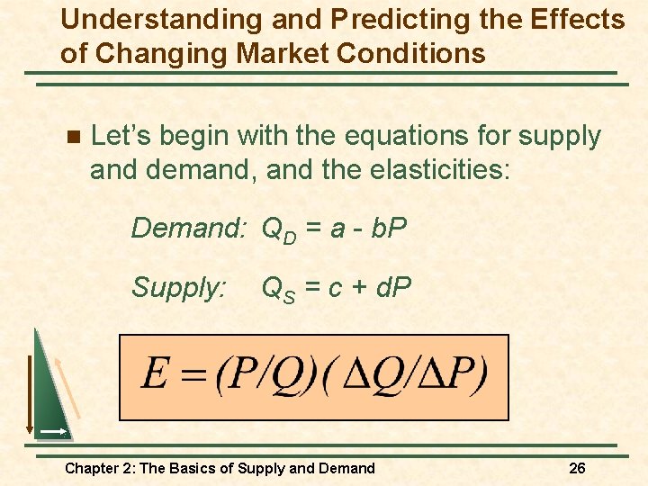
Understanding and Predicting the Effects of Changing Market Conditions n Let’s begin with the equations for supply and demand, and the elasticities: Demand: QD = a - b. P Supply: QS = c + d. P Chapter 2: The Basics of Supply and Demand 26

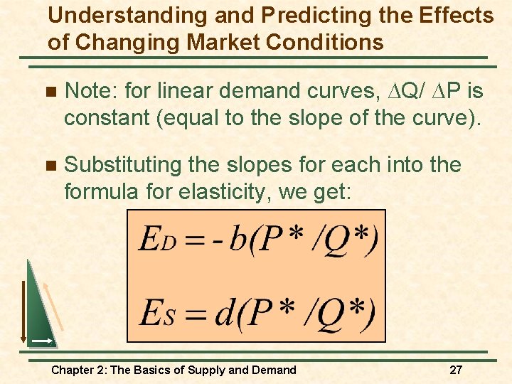
Understanding and Predicting the Effects of Changing Market Conditions n Note: for linear demand curves, ∆Q/ ∆P is constant (equal to the slope of the curve). n Substituting the slopes for each into the formula for elasticity, we get: Chapter 2: The Basics of Supply and Demand 27

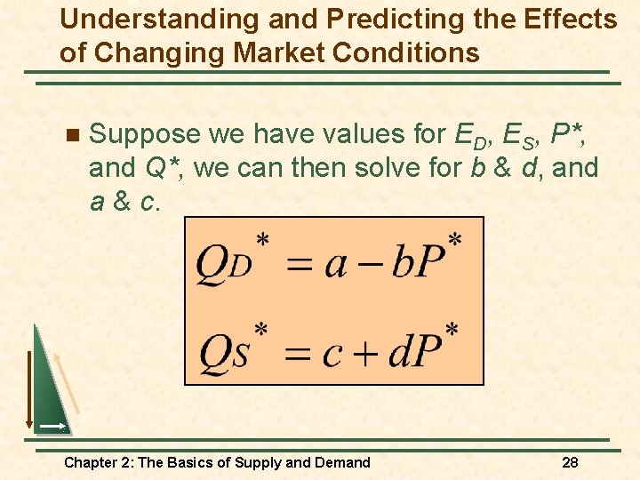
Understanding and Predicting the Effects of Changing Market Conditions n Suppose we have values for ED, ES, P*, and Q*, we can then solve for b & d, and a & c. Chapter 2: The Basics of Supply and Demand 28

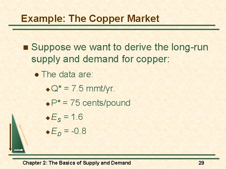
Example: The Copper Market n Suppose we want to derive the long-run supply and demand for copper: l The data are: u Q* = 7. 5 mmt/yr. u P* = 75 cents/pound u ES = 1. 6 u ED = -0. 8 Chapter 2: The Basics of Supply and Demand 29

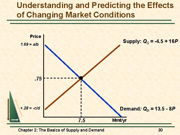
Understanding and Predicting the Effects of Changing Market Conditions Price Supply: QS = -4. 5 + 16 P 1. 69 = a/b . 75 +. 28 = -c/d Demand: QD = 13. 5 - 8 P 7. 5 Chapter 2: The Basics of Supply and Demand Mmt/yr 30

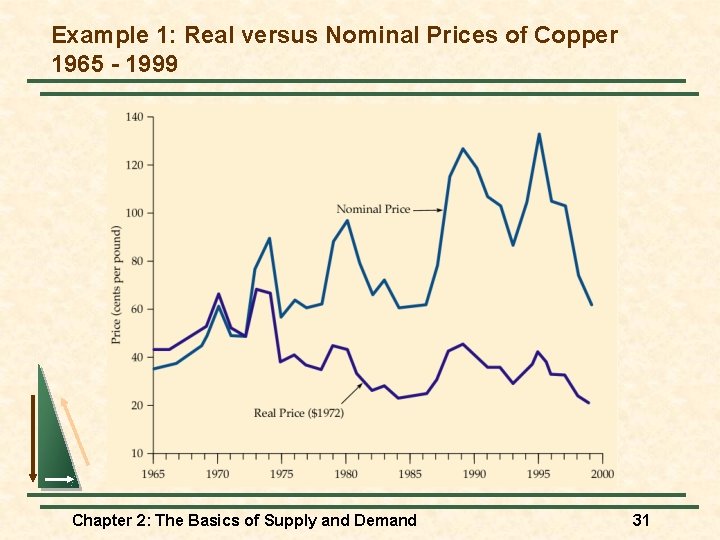
Example 1: Real versus Nominal Prices of Copper 1965 - 1999 Chapter 2: The Basics of Supply and Demand 31

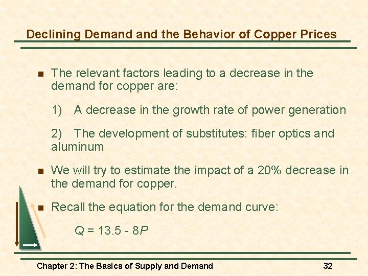
Declining Demand the Behavior of Copper Prices n The relevant factors leading to a decrease in the demand for copper are: 1) A decrease in the growth rate of power generation 2) The development of substitutes: fiber optics and aluminum n We will try to estimate the impact of a 20% decrease in the demand for copper. n Recall the equation for the demand curve: Q = 13. 5 - 8 P Chapter 2: The Basics of Supply and Demand 32

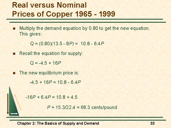
Real versus Nominal Prices of Copper 1965 - 1999 n Multiply the demand equation by 0. 80 to get the new equation. This gives: Q = (0. 80)(13. 5 - 8 P) = 10. 8 - 6. 4 P n Recall the equation for supply: Q = -4. 5 + 16 P n The new equilibrium price is: -4. 5 + 16 P = 10. 8 - 6. 4 P -16 P + 6. 4 P = 10. 8 + 4. 5 P = 15. 3/22. 4 = 68. 3 cents/pound Chapter 2: The Basics of Supply and Demand 33

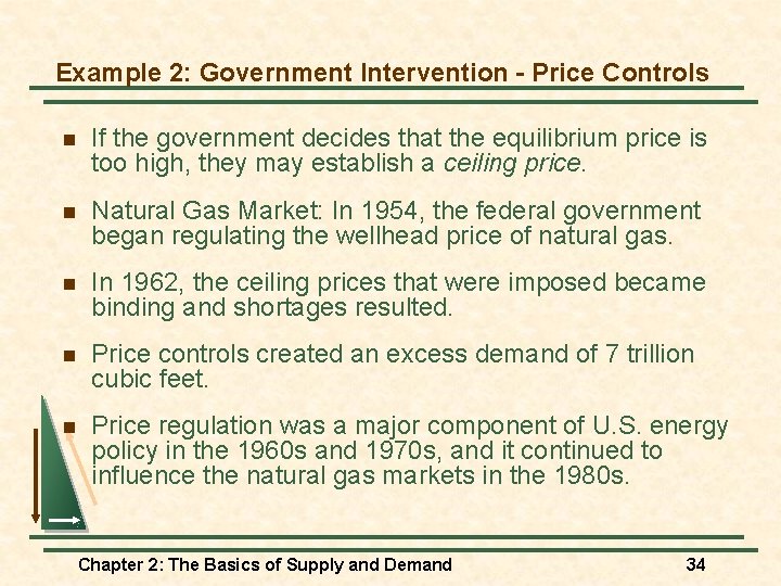
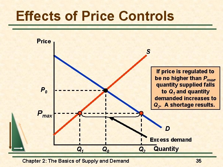
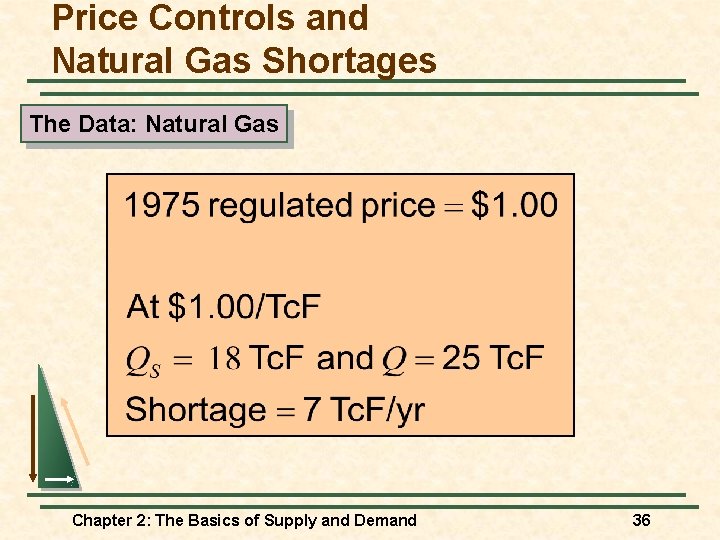
Example 2: Government Intervention - Price Controls n If the government decides that the equilibrium price is too high, they may establish a ceiling price. n Natural Gas Market: In 1954, the federal government began regulating the wellhead price of natural gas. n In 1962, the ceiling prices that were imposed became binding and shortages resulted. n Price controls created an excess demand of 7 trillion cubic feet. n Price regulation was a major component of U. S. energy policy in the 1960 s and 1970 s, and it continued to influence the natural gas markets in the 1980 s. Chapter 2: The Basics of Supply and Demand 34

Effects of Price Controls Price S If price is regulated to be no higher than Pmax, quantity supplied falls to Q 1 and quantity demanded increases to Q 2. A shortage results. P 0 Pmax D Excess demand Q 1 Q 0 Chapter 2: The Basics of Supply and Demand Q 2 Quantity 35

Price Controls and Natural Gas Shortages The Data: Natural Gas Chapter 2: The Basics of Supply and Demand 36