Aggregate Demand Supply Aggregate Demand Curve shows the

Aggregate Demand Supply

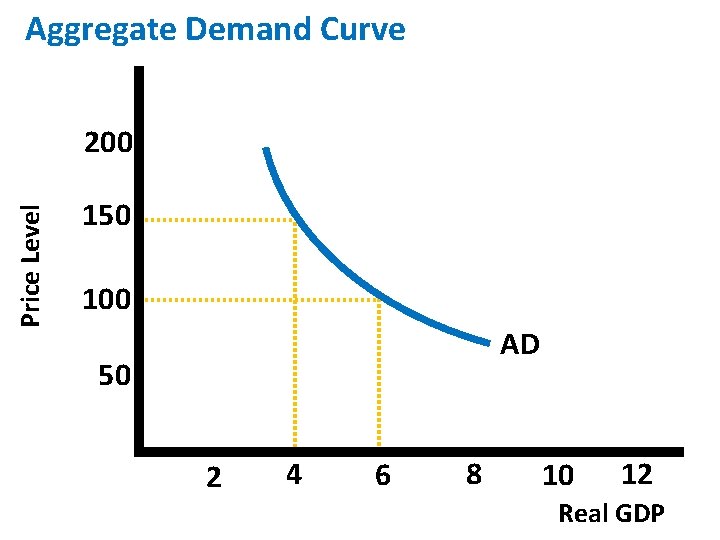
Aggregate Demand Curve shows the level of real GDP purchased by everyone at different price levels during a time period, ceteris paribus The horizontal axis measures the value of final goods and services included in real GDP measured in base year dollars The vertical axis measure is an index of the overall price level, such as the GDP deflator or the CPI Aggregate Demand Curve slopes downward to the right • Real balance wealth effect • Interest rate effect • Net exports effect

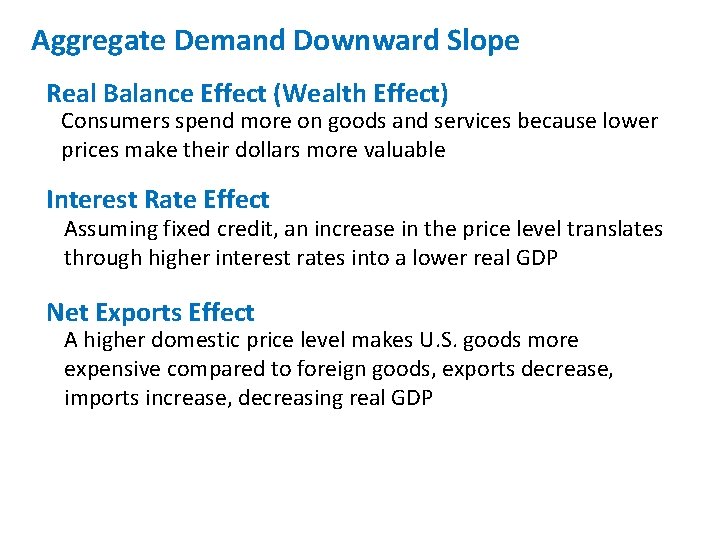
Aggregate Demand Downward Slope Real Balance Effect (Wealth Effect) Consumers spend more on goods and services because lower prices make their dollars more valuable Interest Rate Effect Assuming fixed credit, an increase in the price level translates through higher interest rates into a lower real GDP Net Exports Effect A higher domestic price level makes U. S. goods more expensive compared to foreign goods, exports decrease, imports increase, decreasing real GDP

Aggregate Demand Curve Price Level 200 150 100 AD 50 2 4 6 8 10 12 Real GDP

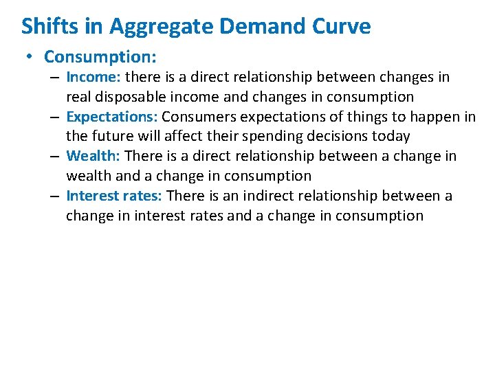
Shifts in Aggregate Demand Curve • Consumption: – Income: there is a direct relationship between changes in real disposable income and changes in consumption – Expectations: Consumers expectations of things to happen in the future will affect their spending decisions today – Wealth: There is a direct relationship between a change in wealth and a change in consumption – Interest rates: There is an indirect relationship between a change in interest rates and a change in consumption

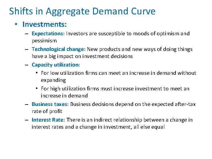
Shifts in Aggregate Demand Curve • Investments: – Expectations: Investors are susceptible to moods of optimism and pessimism – Technological change: New products and new ways of doing things have a big impact on investment decisions – Capacity utilization: • For low utilization firms can meet an increase in demand without expanding • For high utilization firms must increase investment to meet an increase in demand – Business taxes: Business decisions depend on the expected after-tax rate of profit – Interest Rate: There is an indirect relationship between a change in interest rates and a change in investment, all else equal

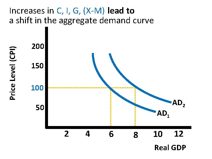
Price Level (CPI) Increases in C, I, G, (X-M) lead to a shift in the aggregate demand curve 200 150 100 50 AD 1 2 4 6 8 10 AD 2 12 Real GDP

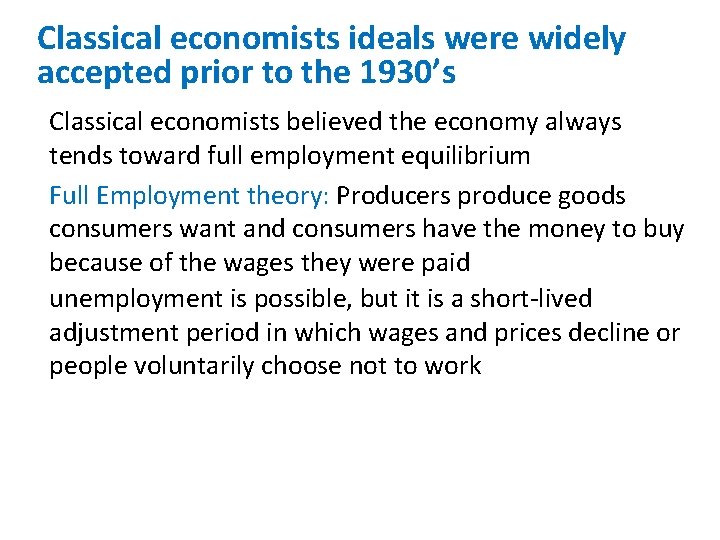
Classical economists ideals were widely accepted prior to the 1930’s Classical economists believed the economy always tends toward full employment equilibrium Full Employment theory: Producers produce goods consumers want and consumers have the money to buy because of the wages they were paid unemployment is possible, but it is a short-lived adjustment period in which wages and prices decline or people voluntarily choose not to work

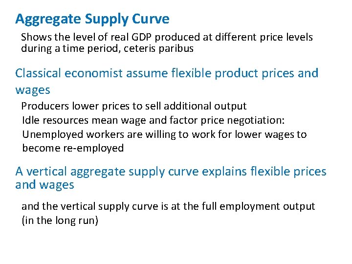
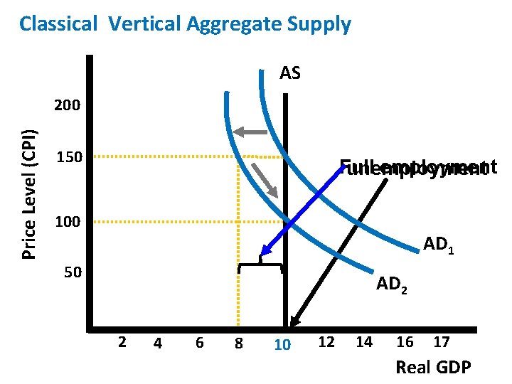
Aggregate Supply Curve Shows the level of real GDP produced at different price levels during a time period, ceteris paribus Classical economist assume flexible product prices and wages Producers lower prices to sell additional output Idle resources mean wage and factor price negotiation: Unemployed workers are willing to work for lower wages to become re-employed A vertical aggregate supply curve explains flexible prices and wages and the vertical supply curve is at the full employment output (in the long run)

Classical Vertical Aggregate Supply AS Price Level (CPI) 200 150 Full employment unemployment 100 AD 1 50 AD 2 2 4 6 8 10 12 14 16 17 Real GDP

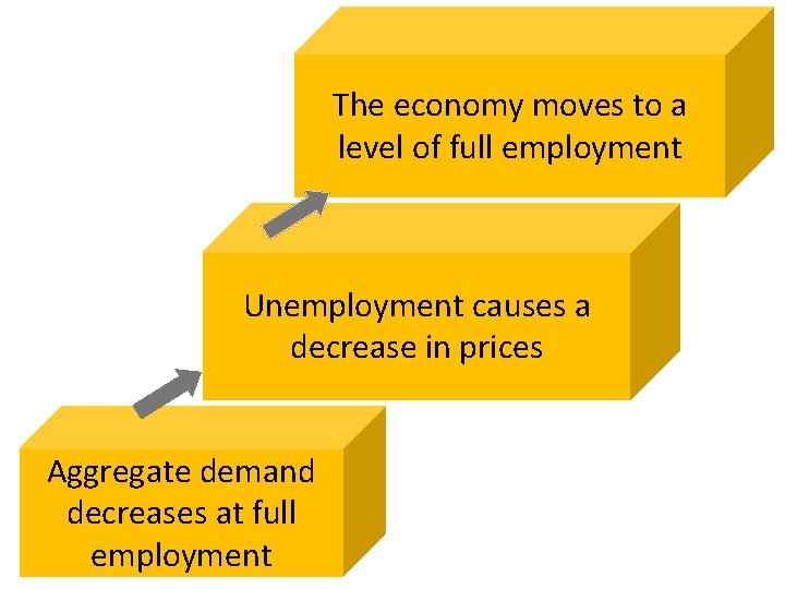
The economy moves to a level of full employment Unemployment causes a decrease in prices Aggregate demand decreases at full employment

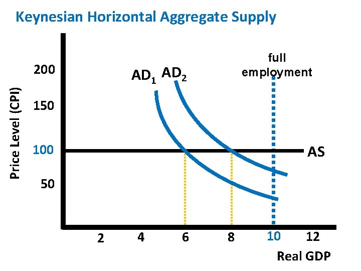
Then comes the Great Depression of the 1930’s Extended long term unemployment for which the classical model did not explain Keynesian Model John Maynard Keynes: A British economist (1883 -1946) who offered an explanation of the Great Depression of the 1930’s Keynes wrote: “The General Theory of Employment, Interest, and Money” Keynes’ theory suggest demand can be forever inadequate for an economy to achieve full employment

Keynesian Horizontal Aggregate Supply Price Level (CPI) 200 full employment AD 1 AD 2 150 100 AS 50 2 4 6 8 10 12 Real GDP

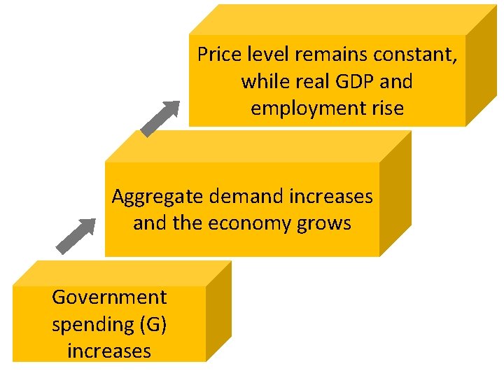
Price level remains constant, while real GDP and employment rise Aggregate demand increases and the economy grows Government spending (G) increases

Understanding the Different Theories Classical economists believe the economy normally operates at its full employment in the long run the price level of products and production costs change by the same percentage in order to maintain full employment Say’s Law: Supply creates it’s own demand Keynesians economists believe that because prices and wages are inflexible the economy can have long term unemployment shifts in aggregate demand will restore a depressed economy to full employment in the long run we’re all dead

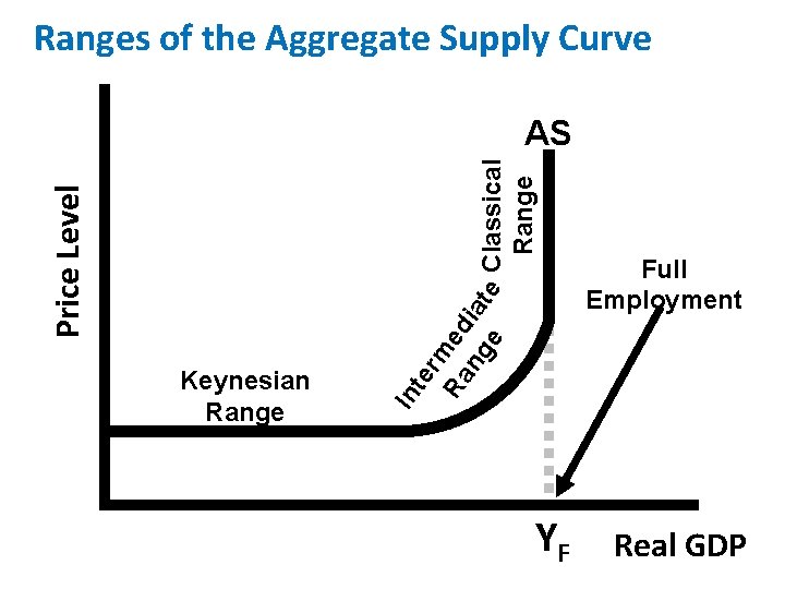
Ranges of the Aggregate Supply Curve te rm Ra ed ng iat e e Keynesian Range Full Employment In Price Level Classical Range AS YF Real GDP

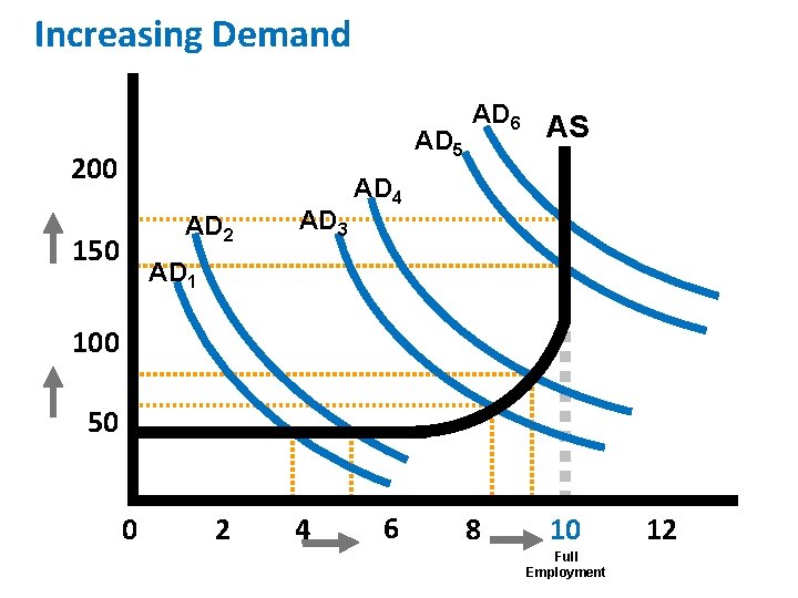
Increasing Demand AD 5 200 AD 2 150 AD 3 AD 6 AS 8 10 AD 4 AD 1 100 50 0 2 4 6 Full Employment 12

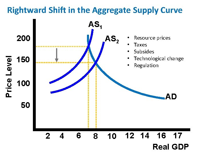
Rightward Shift in the Aggregate Supply Curve AS 1 Price Level 200 AS 2 150 • • • Resource prices Taxes Subsides Technological change Regulation 100 AD 50 2 4 6 8 10 12 14 16 17 Real GDP

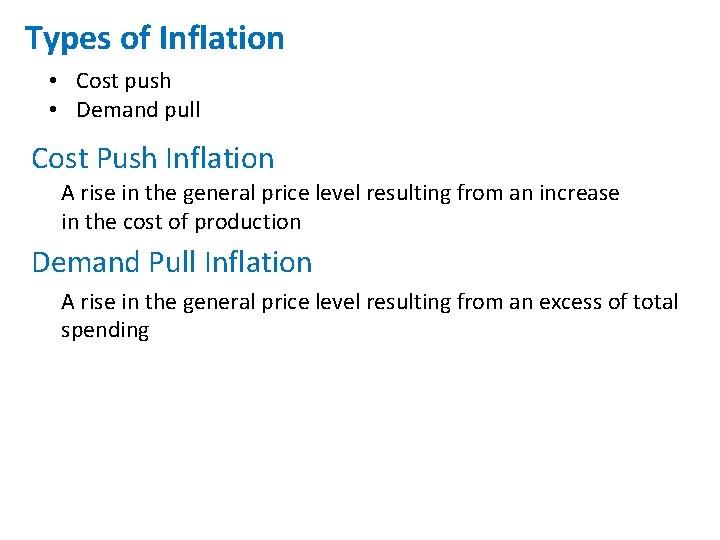
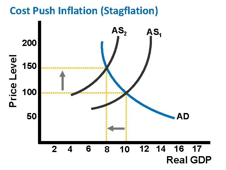
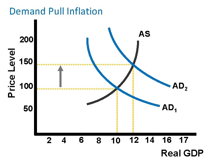
Types of Inflation • Cost push • Demand pull Cost Push Inflation A rise in the general price level resulting from an increase in the cost of production Demand Pull Inflation A rise in the general price level resulting from an excess of total spending

Cost Push Inflation (Stagflation) AS 2 Price Level 200 AS 1 150 100 50 AD 2 4 6 8 10 12 14 16 17 Real GDP

Demand Pull Inflation AS Price Level 200 150 AD 2 100 AD 1 50 2 4 6 8 10 12 14 16 17 Real GDP

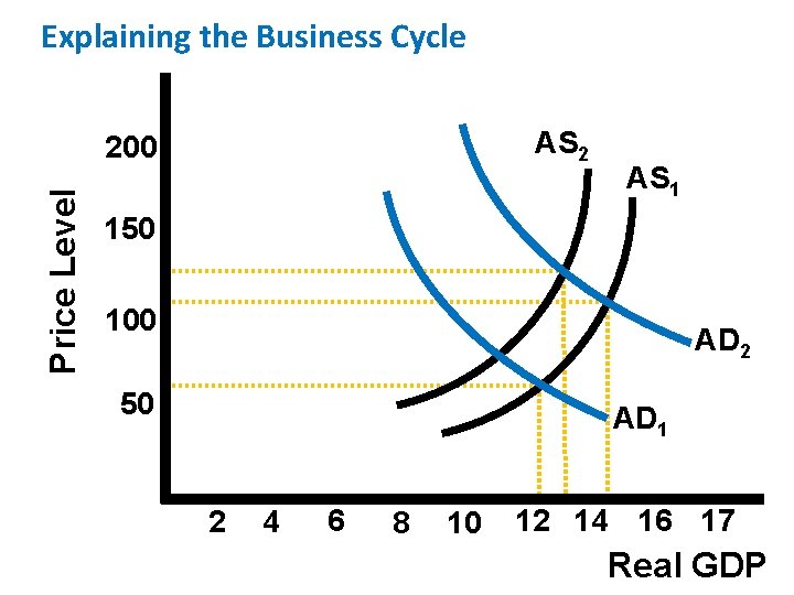
Explaining the Business Cycle AS 2 Price Level 200 AS 1 150 100 AD 2 50 AD 1 2 4 6 8 10 12 14 16 17 Real GDP