Statistical Models in CPT Part II Interpretation Simon

Statistical Models in CPT. Part II: Interpretation Simon J. Mason simon@iri. columbia. edu International Research Institute for Climate and Society The Earth Institute of Columbia University SAWS Training Workshop on the Climate Predictability Tool (CPT) Pretoria, South Africa, 07 – 16 May, 2011

Retaining Principal Components Principal components analysis is specifically designed as a data reduction technique. How many of the new variables should be retained to represent the total variability of the original variables adequately? A stopping rule is required to identify at which point additional principal components are no longer required.

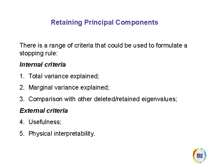
Retaining Principal Components There is a range of criteria that could be used to formulate a stopping rule: Internal criteria 1. Total variance explained; 2. Marginal variance explained; 3. Comparison with other deleted/retained eigenvalues; External criteria 4. Usefulness; 5. Physical interpretability.

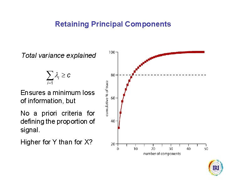
Retaining Principal Components Total variance explained Ensures a minimum loss of information, but No a priori criteria for defining the proportion of signal. Higher for Y than for X?

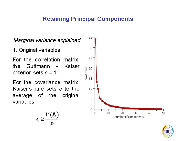
Retaining Principal Components Marginal variance explained Ensures that each component explains a substantial proportion of the total variance. Choice of c?

Retaining Principal Components Marginal variance explained 1. Original variables For the correlation matrix, the Guttmann - Kaiser criterion sets c = 1. For the covariance matrix, Kaiser’s rule sets c to the average of the original variables:

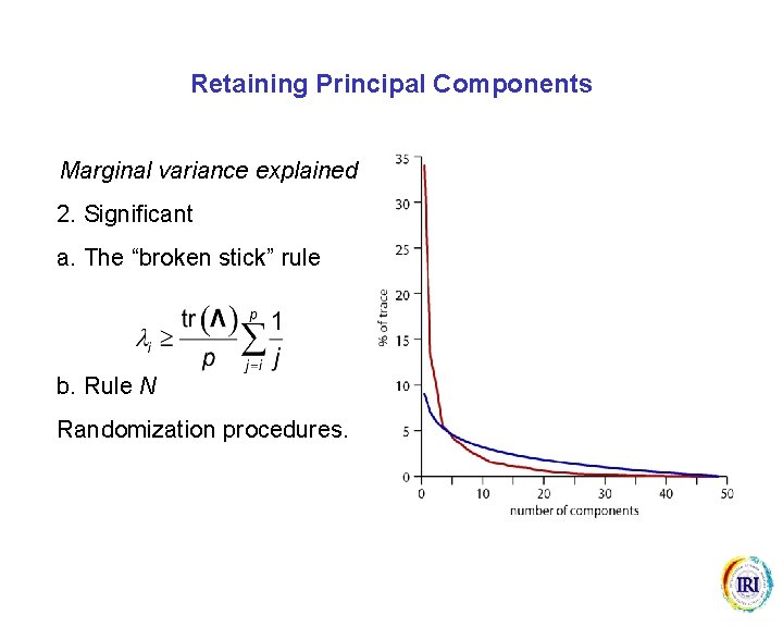
Retaining Principal Components Marginal variance explained 2. Significant a. The “broken stick” rule b. Rule N Randomization procedures.

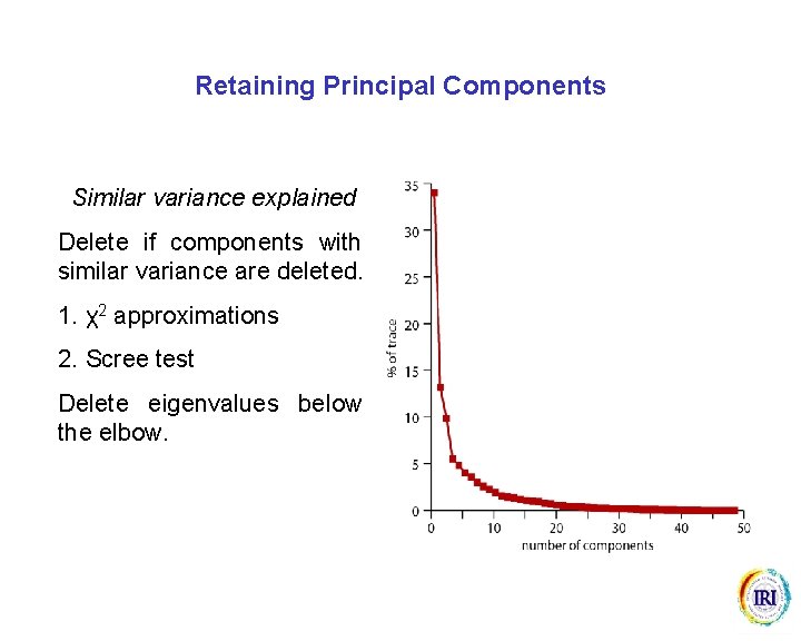
Retaining Principal Components Similar variance explained Delete if components with similar variance are deleted. 1. χ2 approximations 2. Scree test Delete eigenvalues below the elbow.

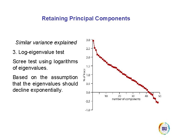
Retaining Principal Components Similar variance explained 3. Log-eigenvalue test Scree test using logarithms of eigenvalues. Based on the assumption that the eigenvalues should decline exponentially.

Retaining Principal Components Usefulness If principal components are to be used in other applications, retain the number that gives the best results. Use cross-validation. Perhaps retain subsets that do not necessarily include the first few components. Possibly subject to sampling errors, especially subset selection.

Retaining Principal Components Physical interpretability 1. Time scores Do the time scores differ from white noise? 2. Spatial loadings Loadings identify “modes” of variability.

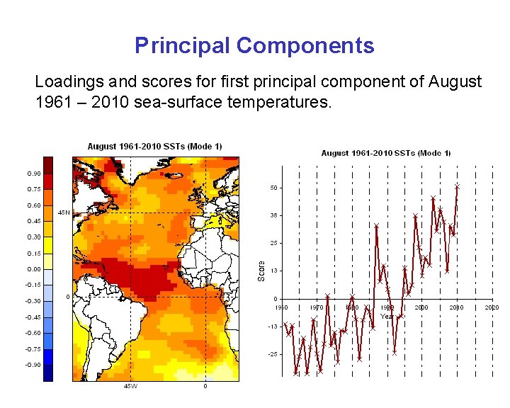
Principal Components Loadings and scores for first principal component of August 1961 – 2010 sea-surface temperatures.

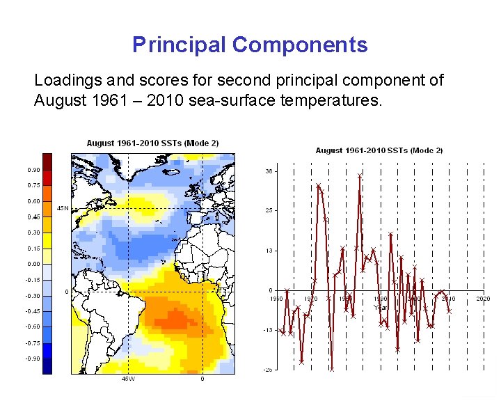
Principal Components Loadings and scores for second principal component of August 1961 – 2010 sea-surface temperatures.

Interpreting the Principal Components Principal components are notoriously difficult to interpret physically. The weights are defined to maximize the variance, not maximize the interpretability! With spatial data (including climate data) the interpretation becomes even more difficult because there are geometric controls on the correlations between the data points.

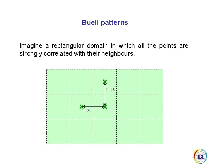
Buell patterns Imagine a rectangular domain in which all the points are strongly correlated with their neighbours.

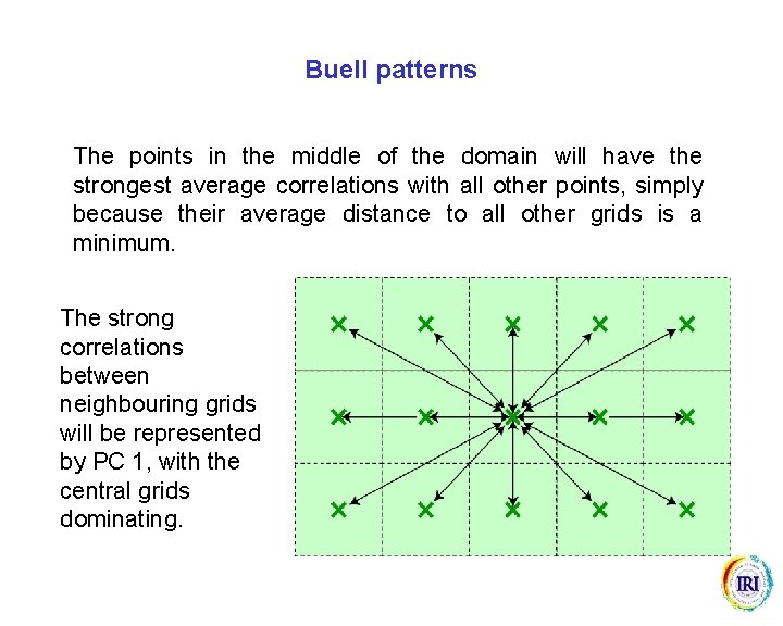
Buell patterns The points in the middle of the domain will have the strongest average correlations with all other points, simply because their average distance to all other grids is a minimum. The strong correlations between neighbouring grids will be represented by PC 1, with the central grids dominating.

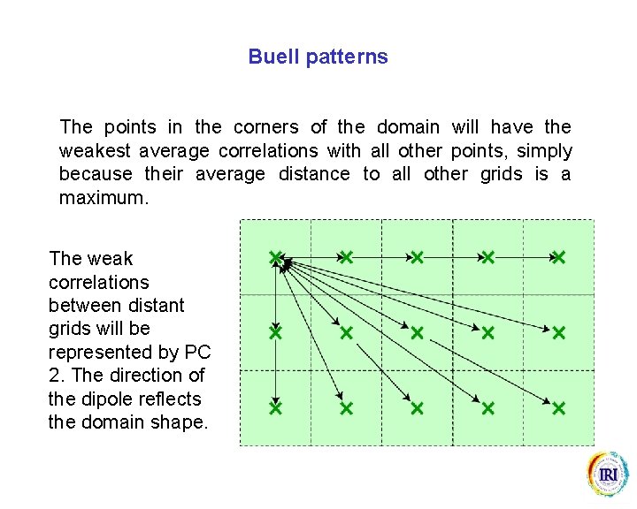
Buell patterns The points in the corners of the domain will have the weakest average correlations with all other points, simply because their average distance to all other grids is a maximum. The weak correlations between distant grids will be represented by PC 2. The direction of the dipole reflects the domain shape.

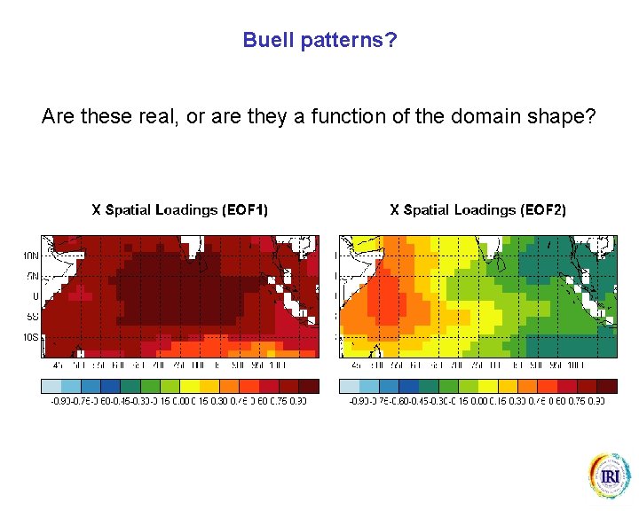
Buell patterns? Are these real, or are they a function of the domain shape?

Buell patterns Because of domain shape dependency: 1. the first PC frequently indicates positive loadings with strongest values in the centre of the domain; 2. the second PC frequently indicates negative loadings on one side and positive loadings on the other side in the direction of the longest dimension of the domain. Similar kinds of problems arise when using: 1. gridded data with converging longitudes, or simply with longitude spacing different from latitude spacing; 2. station data.

Rotation The principal component weights are defined to maximize the variance, not maximize the interpretability! The weights could be redefined to meet alternative criteria. Rotation is sometimes performed to maximize the weights of as many metrics as possible, and to minimize the weights of the others. An objective of rotation is to attain simple structure: 1. weights are either close to zero or close to one; 2. variables have high weights on only one component.

Rotation Commonly used rotation procedures include: • Varimax – maximises the variance of the squared loadings. • Quartimin – oblique rotation • Procrustes – maximises the similarity between one set of loadings and a target set. Can be orthogonal or oblique.

Rotation does NOT solve Buell pattern problems, nor station and uneven gridded data problems, it only reduces them. What if a mode does not have simple structure – for example, a general warming trend? These problems are only of concern for interpretation. Rotation may be redundant if the principal components are used as input into some other procedures.

Buell Patterns in CCA