School of Environmental Engineering EAT 342 Noise Pollution

| School of Environmental Engineering EAT 342: Noise Pollution Control Chapter 2: Noise and Vibration By: Dr. Sara Yasina Yusuf

Course Objectives & Learning Objectives • This chapter reflects CO 2: – Ability of defining the properties of sound, quantifying the noise levels and decibel as well as to characterize the noise. • Learning Objectives for the chapter: – LO-1: DISCUSS the basic physics of sound and CALCULATE the speed of sound, sound pressure, frequency and wavelength. – LO-2: DEFINE sound scale in decibel. – LO-3: DIFFERENTIATE and CALCULATE the Sound Power Level, Sound Intensity and Sound Pressure Level. – LO-4: CALCULATE the Average Sound Power Level, summation of sound pressure using formula, table and graph. – LO-5: SKETCH normal sound wave spectrum with relevant units – LO-6: LIST THREE (3) methods of noise analyses, i. e. , phone, octave bands and weighted sound pressure and definition of each. | School of Environmental Engineering 2

Chapter’s Content 1. The basic physics of sound – – – Sound and types of sound Speed of sound Sound pressure Frequency Wavelength – 3. Noise measurement – – 2. Characteristics of noise and Desibel scale – – Frequency and Loudness Sound level and decibel scale Weighting networks Octave bands | School of Environmental Engineering Averaging sound pressure levels – – Field Equipment and Accessories Permanent Outdoor Microphone Units Tape Recorders The Measurement Reports 3

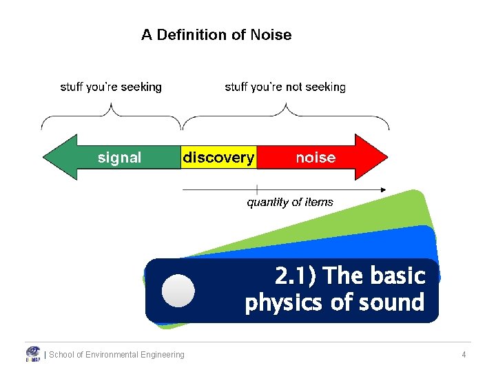
2. 1) The basic physics of sound | School of Environmental Engineering 4

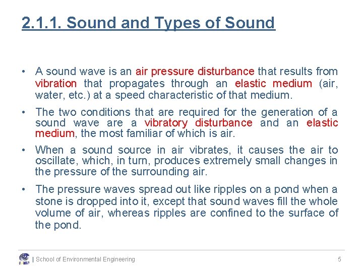
2. 1. 1. Sound and Types of Sound • A sound wave is an air pressure disturbance that results from vibration that propagates through an elastic medium (air, water, etc. ) at a speed characteristic of that medium. • The two conditions that are required for the generation of a sound wave are a vibratory disturbance and an elastic medium, the most familiar of which is air. • When a sound source in air vibrates, it causes the air to oscillate, which, in turn, produces extremely small changes in the pressure of the surrounding air. • The pressure waves spread out like ripples on a pond when a stone is dropped into it, except that sound waves fill the whole volume of air, whereas ripples are confined to the surface of the pond. | School of Environmental Engineering 5

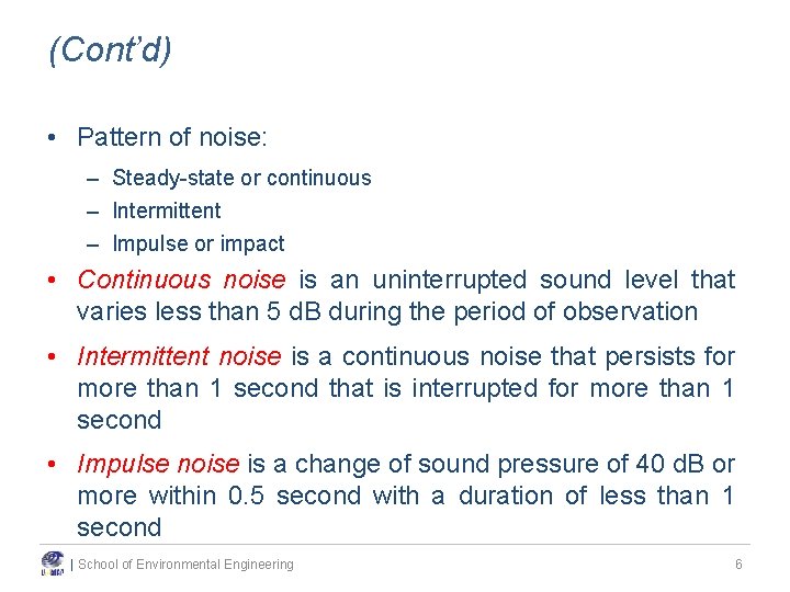
(Cont’d) • Pattern of noise: – Steady-state or continuous – Intermittent – Impulse or impact • Continuous noise is an uninterrupted sound level that varies less than 5 d. B during the period of observation • Intermittent noise is a continuous noise that persists for more than 1 second that is interrupted for more than 1 second • Impulse noise is a change of sound pressure of 40 d. B or more within 0. 5 second with a duration of less than 1 second | School of Environmental Engineering 6

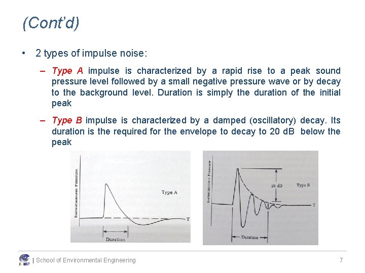
(Cont’d) • 2 types of impulse noise: – Type A impulse is characterized by a rapid rise to a peak sound pressure level followed by a small negative pressure wave or by decay to the background level. Duration is simply the duration of the initial peak – Type B impulse is characterized by a damped (oscillatory) decay. Its duration is the required for the envelope to decay to 20 d. B below the peak | School of Environmental Engineering 7

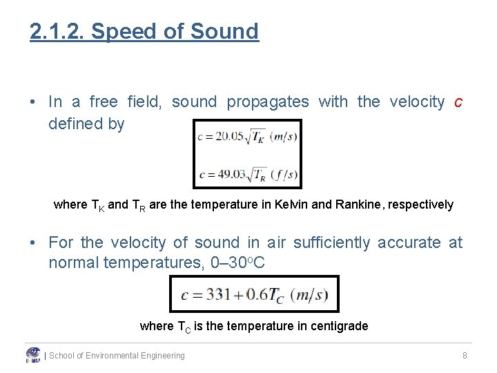
2. 1. 2. Speed of Sound • In a free field, sound propagates with the velocity c defined by where TK and TR are the temperature in Kelvin and Rankine, respectively • For the velocity of sound in air sufficiently accurate at normal temperatures, 0– 30 o. C where TC is the temperature in centigrade | School of Environmental Engineering 8

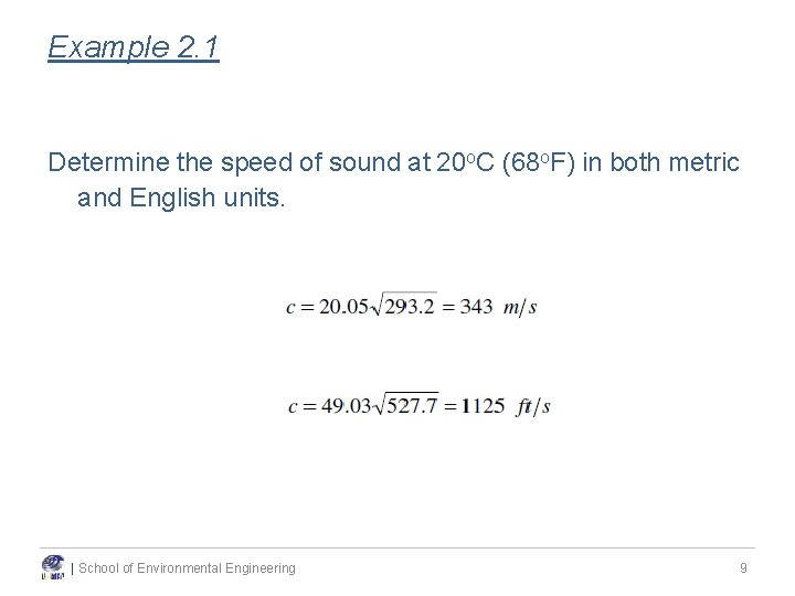
Example 2. 1 Determine the speed of sound at 20 o. C (68 o. F) in both metric and English units. | School of Environmental Engineering 9

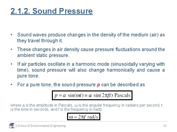
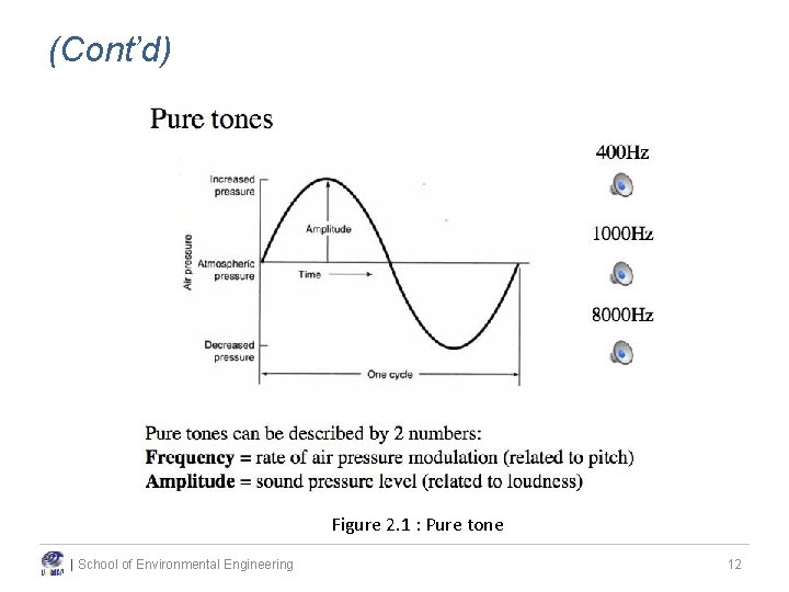
2. 1. 2. Sound Pressure • Sound waves produce changes in the density of the medium (air) as they travel through it. • These changes in air density cause pressure fluctuations around the ambient static pressure. • If air particles oscillate in a harmonic mode (sinusoidally varying with time), sound pressure will also change harmonically and cause a pure tone. • For a pure tone, the sound pressure p can be described as where a is the amplitude in Pascals, ω is the angular frequency in radians per second, t is the time in seconds, and f is the frequency in hertz. | School of Environmental Engineering 10

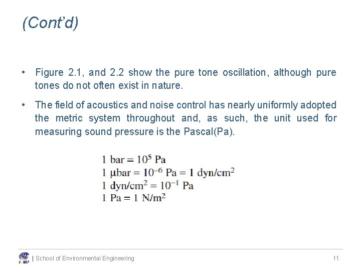
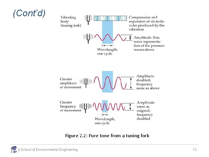
(Cont’d) • Figure 2. 1, and 2. 2 show the pure tone oscillation, although pure tones do not often exist in nature. • The field of acoustics and noise control has nearly uniformly adopted the metric system throughout and, as such, the unit used for measuring sound pressure is the Pascal(Pa). | School of Environmental Engineering 11

(Cont’d) Figure 2. 1 : Harmonic oscillation of pressure Figure 2. 1 : Pure tone | School of Environmental Engineering 12

(Cont’d) Figure 2. 2: Pure tone from a tuning fork | School of Environmental Engineering 13

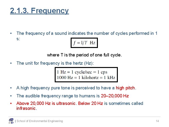
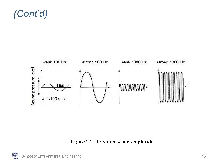
2. 1. 3. Frequency • The frequency of a sound indicates the number of cycles performed in 1 s: where T is the period of one full cycle. • The unit for frequency is the hertz (Hz): • A high frequency pure tone is perceived to have a high pitch. • The audible frequency range to humans is 20– 20, 000 Hz • Above 20, 000 Hz is ultrasonic. Below 20 Hz is sometimes called infrasonic. | School of Environmental Engineering 14

(Cont’d) Figure 2. 3 : Frequency and amplitude | School of Environmental Engineering 15

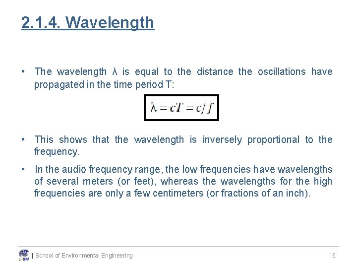
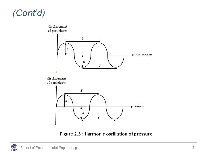
2. 1. 4. Wavelength • The wavelength λ is equal to the distance the oscillations have propagated in the time period T: • This shows that the wavelength is inversely proportional to the frequency. • In the audio frequency range, the low frequencies have wavelengths of several meters (or feet), whereas the wavelengths for the high frequencies are only a few centimeters (or fractions of an inch). | School of Environmental Engineering 16

(Cont’d) Figure 2. 5 : Harmonic oscillation of pressure | School of Environmental Engineering 17

2). 2 | School of Environmental Engineering f o cs ise i t is No r te c ra a Ch 18

2. 2. 1. Frequency and Loudness • There are two important characteristics of sound or noise - frequency and loudness. • The number of pressure variations per second is called the frequency of sound, and is measured in Hertz (Hz) which is defined as cycles per second. • The higher the frequency, the more high-pitched a sound is perceived. • Frequency Pitch • Amplitude Loudness | School of Environmental Engineering 19

Example 2. 2 Determine the wavelength of a 125 -Hz and an 8000 -Hz tone at 20 o. C (68 o. F) in both metric and English units. | School of Environmental Engineering 20

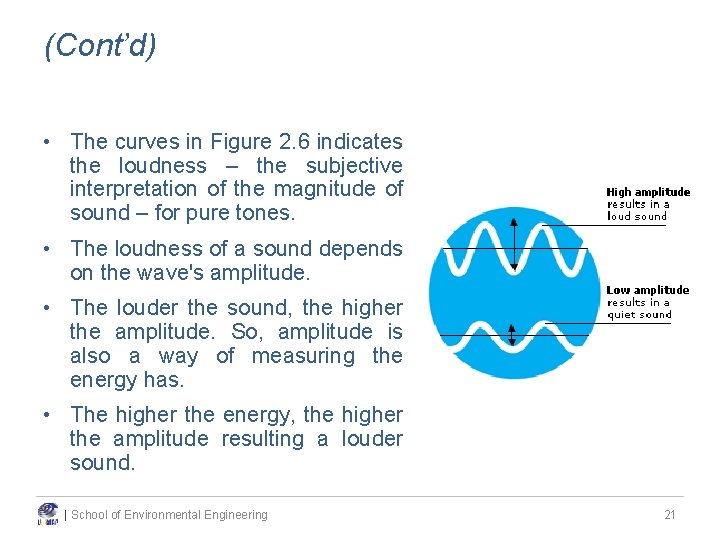
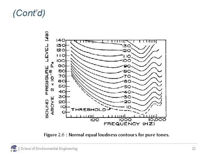
(Cont’d) • The curves in Figure 2. 6 indicates the loudness – the subjective interpretation of the magnitude of sound – for pure tones. • The loudness of a sound depends on the wave's amplitude. • The louder the sound, the higher the amplitude. So, amplitude is also a way of measuring the energy has. • The higher the energy, the higher the amplitude resulting a louder sound. | School of Environmental Engineering 21

(Cont’d) Figure 2. 6 : Normal equal loudness contours for pure tones. | School of Environmental Engineering 22

(Cont’d) • For example, as can be seen in Fig. 2. 6, the threshold of hearing at 1000 Hz is about 4 d. B. • A 20 -Hz tone must have a sound pressure level about 70 d. B higher than a tone at 1000 Hz in order for a person just to hear the tone. • The curves also indicated the loudness—the subjective interpretation of the magnitude of sound—for pure tones. • The units describing loudness are called phons. By definition, the phon is equal to the sound pressure level (in d. B) reference to 20 μPa of an equally loud 1000 -Hz tone. • Pain will occur when the loudness exceeds 120 phons. | School of Environmental Engineering 23

2. 2. 2. Sound Level and Decibel Scale • As explained previously, sound is measured in unit of pressure and normally referred in Pascal and Newton per meter square or “psi”. • The lowest audible sound pressure is 0. 00002 Pa (0 r 20 x 10 -6 Pa equivalent 20 μPa). • This value is very low as compared to sound emitted from a taking off jet i. e. , 200 Pa. Note that the range of difference between these is so great. • Therefore, a scale based on the logarithm of the ratios of the measured quantities is used. • Measurements on this scale are called levels. | School of Environmental Engineering 24

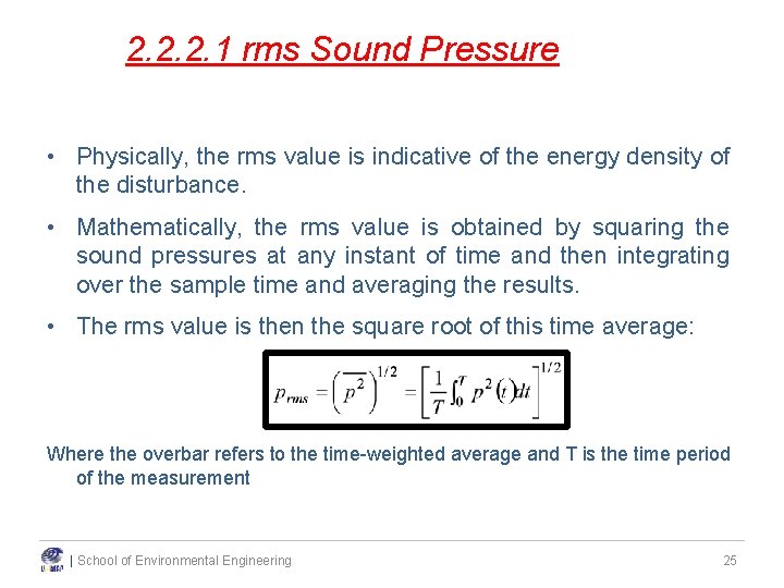
2. 2. 2. 1 rms Sound Pressure • Physically, the rms value is indicative of the energy density of the disturbance. • Mathematically, the rms value is obtained by squaring the sound pressures at any instant of time and then integrating over the sample time and averaging the results. • The rms value is then the square root of this time average: Where the overbar refers to the time-weighted average and T is the time period of the measurement | School of Environmental Engineering 25

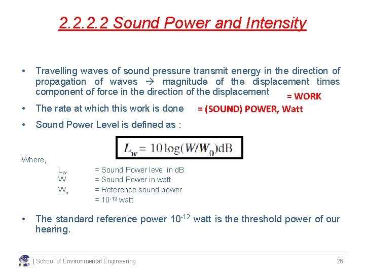
2. 2 Sound Power and Intensity • Travelling waves of sound pressure transmit energy in the direction of propagation of waves magnitude of the displacement times component of force in the direction of the displacement = WORK • The rate at which this work is done • Sound Power Level is defined as : = (SOUND) POWER, Watt Where, Lw W Wo • = Sound Power level in d. B = Sound Power in watt = Reference sound power = 10 -12 watt The standard reference power 10 -12 watt is the threshold power of our hearing. | School of Environmental Engineering 26

(Cont’d) • Please note that, direct reading of sound power is not possible. Sound Level meter functions by measuring sound pressure or the difference in pressure due to vibration of air molecule, compared to 1 atm. • Equation 2. 2 describes the power emitted from a noise source. • For example, when we speak, our voice vibrates the air molecule causing the pressure to increase and a sound power is generated. • What is measured by the instrument is the pressure. • Development of sound measurement instruments are currently based on the measurement of pressure and not the power. | School of Environmental Engineering 27

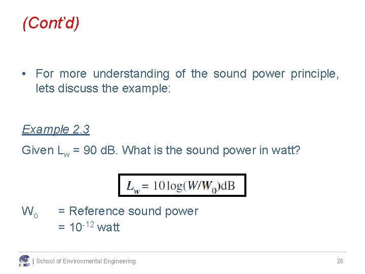
(Cont’d) • For more understanding of the sound power principle, lets discuss the example: Example 2. 3 Given Lw = 90 d. B. What is the sound power in watt? Wo = Reference sound power = 10 -12 watt | School of Environmental Engineering 28

(Cont’d) Tutorial Calculate Sound Power for given noise sources of 40 d. B and 140 d. B. Which one is higher? | School of Environmental Engineering 29

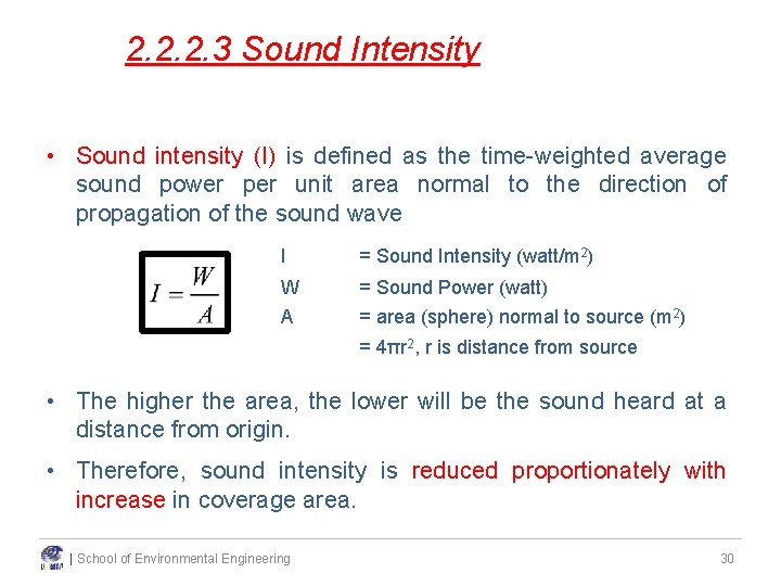
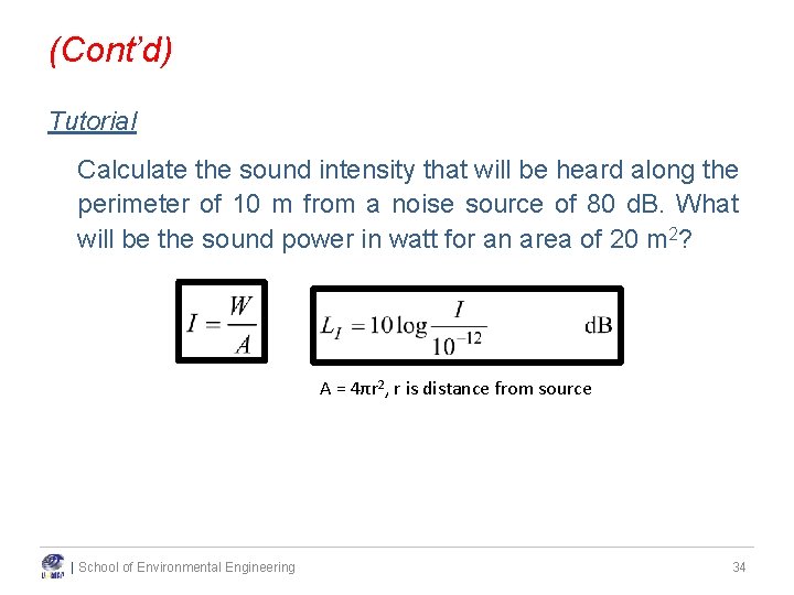
2. 2. 2. 3 Sound Intensity • Sound intensity (I) is defined as the time-weighted average sound power per unit area normal to the direction of propagation of the sound wave I = Sound Intensity (watt/m 2) W = Sound Power (watt) A = area (sphere) normal to source (m 2) = 4πr 2, r is distance from source • The higher the area, the lower will be the sound heard at a distance from origin. • Therefore, sound intensity is reduced proportionately with increase in coverage area. | School of Environmental Engineering 30

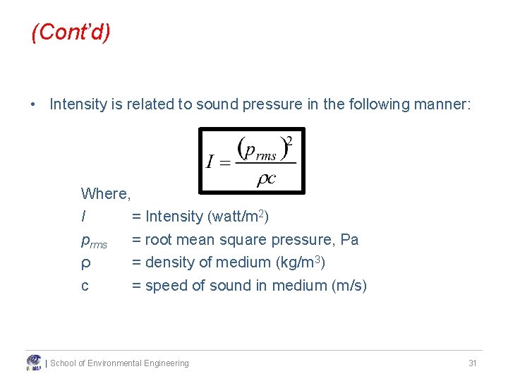
(Cont’d) • Intensity is related to sound pressure in the following manner: Where, I = Intensity (watt/m 2) prms = root mean square pressure, Pa ρ = density of medium (kg/m 3) c = speed of sound in medium (m/s) | School of Environmental Engineering 31

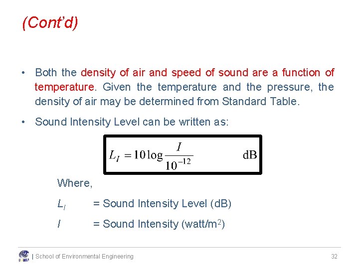
(Cont’d) • Both the density of air and speed of sound are a function of temperature. Given the temperature and the pressure, the density of air may be determined from Standard Table. • Sound Intensity Level can be written as: Where, LI = Sound Intensity Level (d. B) I = Sound Intensity (watt/m 2) | School of Environmental Engineering 32

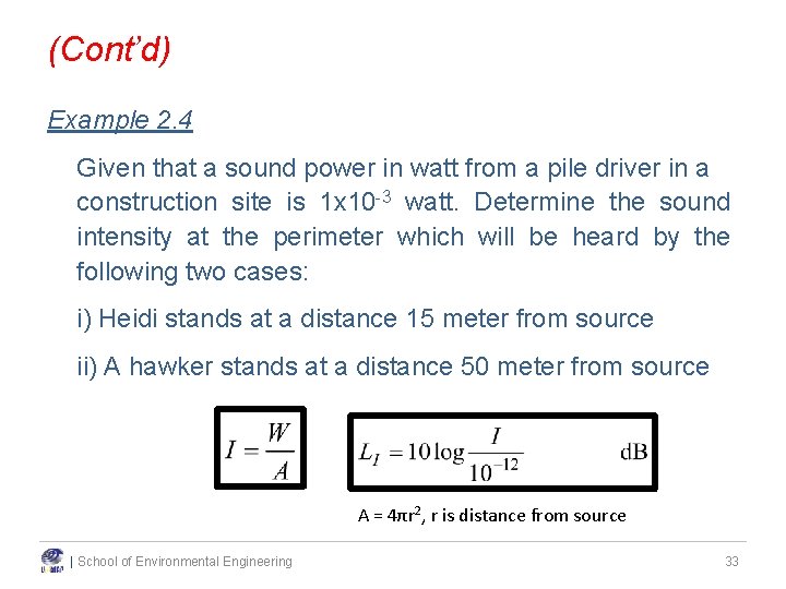
(Cont’d) Example 2. 4 Given that a sound power in watt from a pile driver in a construction site is 1 x 10 -3 watt. Determine the sound intensity at the perimeter which will be heard by the following two cases: i) Heidi stands at a distance 15 meter from source ii) A hawker stands at a distance 50 meter from source A = 4πr 2, r is distance from source | School of Environmental Engineering 33

(Cont’d) Tutorial Calculate the sound intensity that will be heard along the perimeter of 10 m from a noise source of 80 d. B. What will be the sound power in watt for an area of 20 m 2? A = 4πr 2, r is distance from source | School of Environmental Engineering 34

| School of Environmental Engineering 35

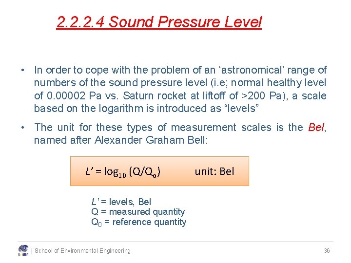
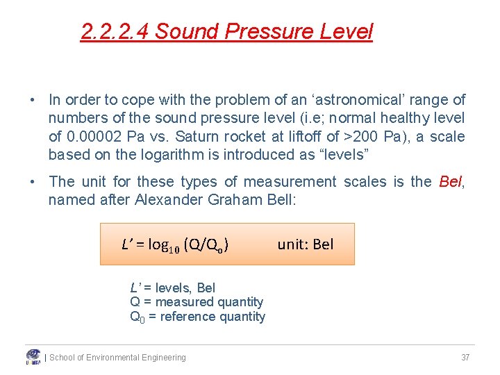
2. 2. 2. 4 Sound Pressure Level • In order to cope with the problem of an ‘astronomical’ range of numbers of the sound pressure level (i. e; normal healthy level of 0. 00002 Pa vs. Saturn rocket at liftoff of >200 Pa), a scale based on the logarithm is introduced as “levels” • The unit for these types of measurement scales is the Bel, named after Alexander Graham Bell: L’ = log 10 (Q/Qo) unit: Bel L’ = levels, Bel Q = measured quantity Q 0 = reference quantity | School of Environmental Engineering 36

2. 2. 2. 4 Sound Pressure Level • In order to cope with the problem of an ‘astronomical’ range of numbers of the sound pressure level (i. e; normal healthy level of 0. 00002 Pa vs. Saturn rocket at liftoff of >200 Pa), a scale based on the logarithm is introduced as “levels” • The unit for these types of measurement scales is the Bel, named after Alexander Graham Bell: L’ = log 10 (Q/Qo) unit: Bel L’ = levels, Bel Q = measured quantity Q 0 = reference quantity | School of Environmental Engineering 37

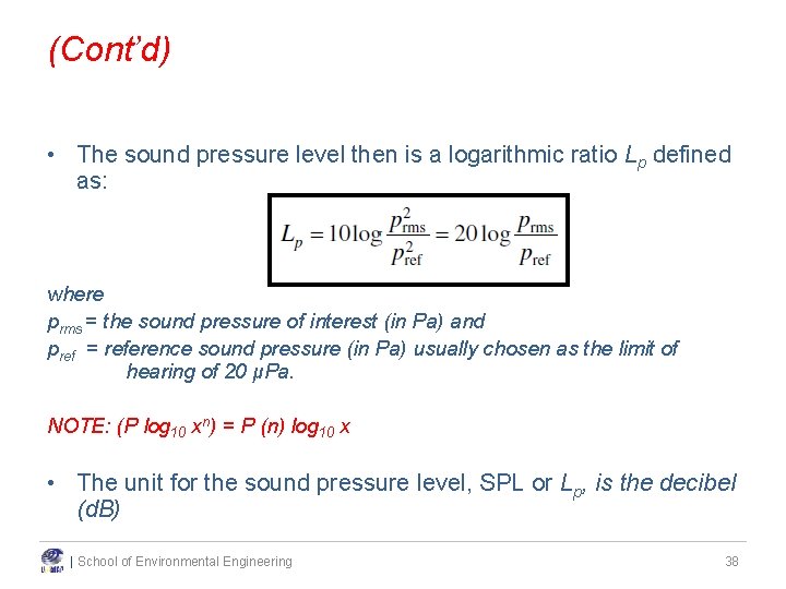
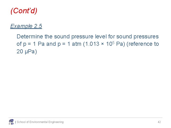
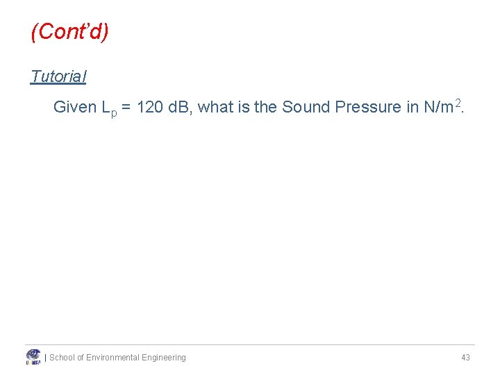
(Cont’d) • The sound pressure level then is a logarithmic ratio Lp defined as: where prms = the sound pressure of interest (in Pa) and pref = reference sound pressure (in Pa) usually chosen as the limit of hearing of 20 μPa. NOTE: (P log 10 xn) = P (n) log 10 x • The unit for the sound pressure level, SPL or Lp, is the decibel (d. B) | School of Environmental Engineering 38

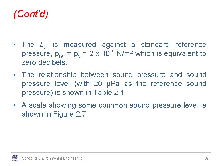
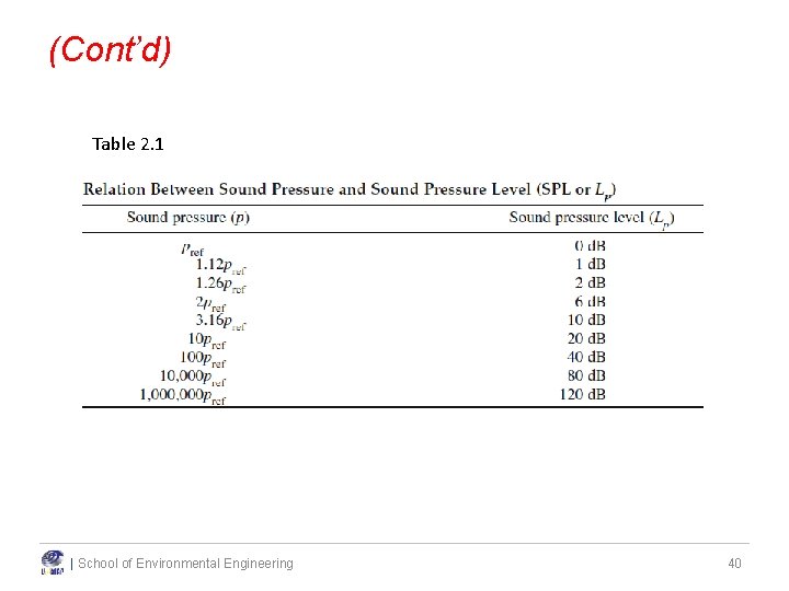
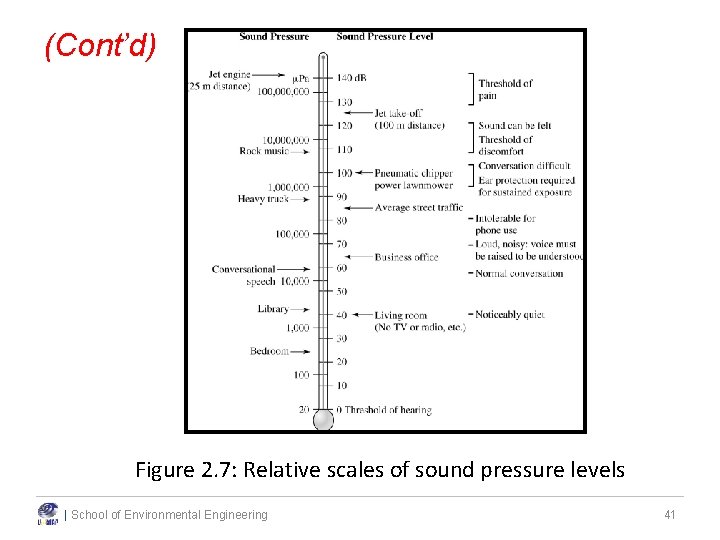
(Cont’d) • The LP is measured against a standard reference pressure, pref = po = 2 x 10 -5 N/m 2 which is equivalent to zero decibels. • The relationship between sound pressure and sound pressure level (with 20 μPa as the reference sound pressure) is shown in Table 2. 1. • A scale showing some common sound pressure level is shown in Figure 2. 7. | School of Environmental Engineering 39

(Cont’d) Table 2. 1 | School of Environmental Engineering 40

(Cont’d) Figure 2. 7: Relative scales of sound pressure levels | School of Environmental Engineering 41

(Cont’d) Example 2. 5 Determine the sound pressure level for sound pressures of p = 1 Pa and p = 1 atm (1. 013 × 105 Pa) (reference to 20 μPa) | School of Environmental Engineering 42

(Cont’d) Tutorial Given Lp = 120 d. B, what is the Sound Pressure in N/m 2. | School of Environmental Engineering 43

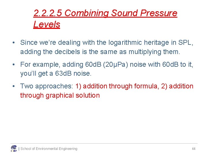
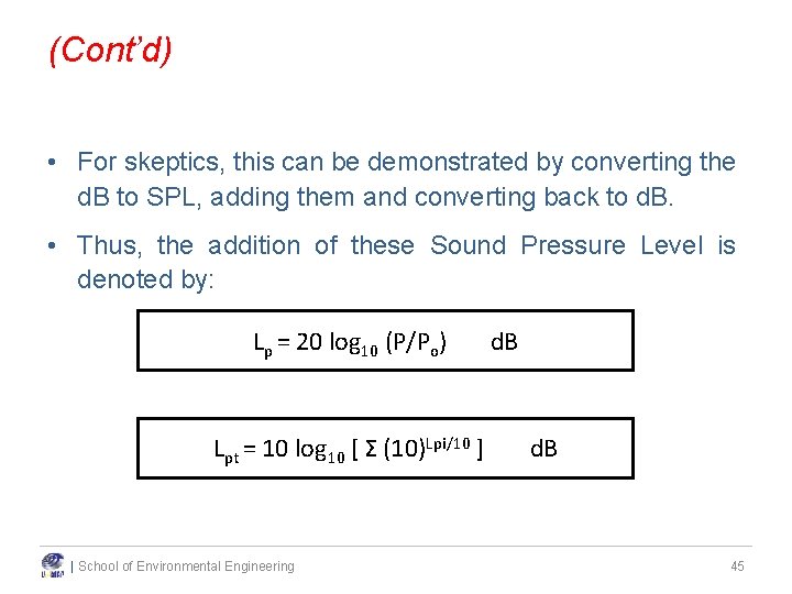
2. 2. 2. 5 Combining Sound Pressure Levels • Since we’re dealing with the logarithmic heritage in SPL, adding the decibels is the same as multiplying them. • For example, adding 60 d. B (20µPa) noise with 60 d. B to it, you’ll get a 63 d. B noise. • Two approaches: 1) addition through formula, 2) addition through graphical solution | School of Environmental Engineering 44

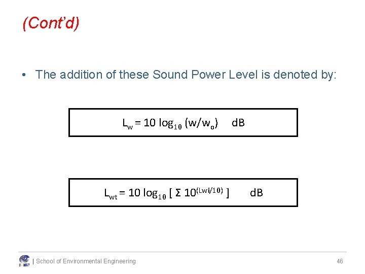
(Cont’d) • For skeptics, this can be demonstrated by converting the d. B to SPL, adding them and converting back to d. B. • Thus, the addition of these Sound Pressure Level is denoted by: Lp = 20 log 10 (P/Po) Lpt = 10 log 10 [ Σ (10)Lpi/10 ] | School of Environmental Engineering d. B 45

(Cont’d) • The addition of these Sound Power Level is denoted by: Lw = 10 log 10 (w/wo) Lwt = 10 log 10 [ Σ 10(Lwi/10) ] | School of Environmental Engineering d. B 46

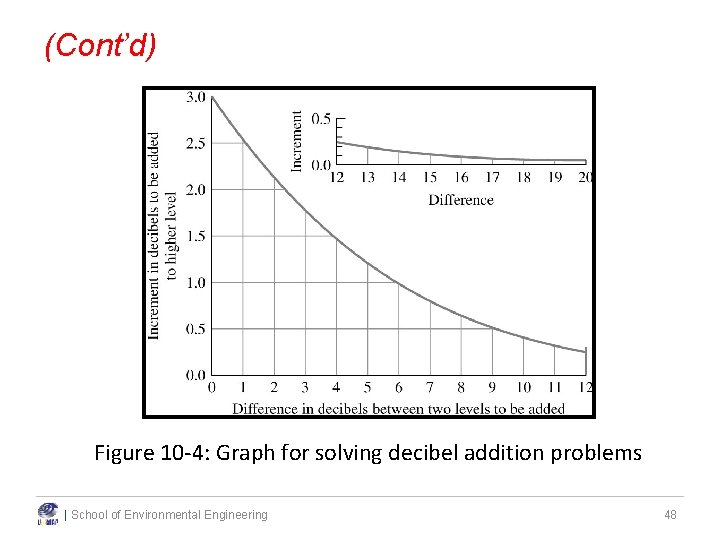
(Cont’d) • A graphical solution for this type of problem is provided as in Figure 2. 8. • For noise pollution work, results should be reported to the nearest whole number. | School of Environmental Engineering 47

(Cont’d) Figure 10 -4: Graph for solving decibel addition problems | School of Environmental Engineering 48

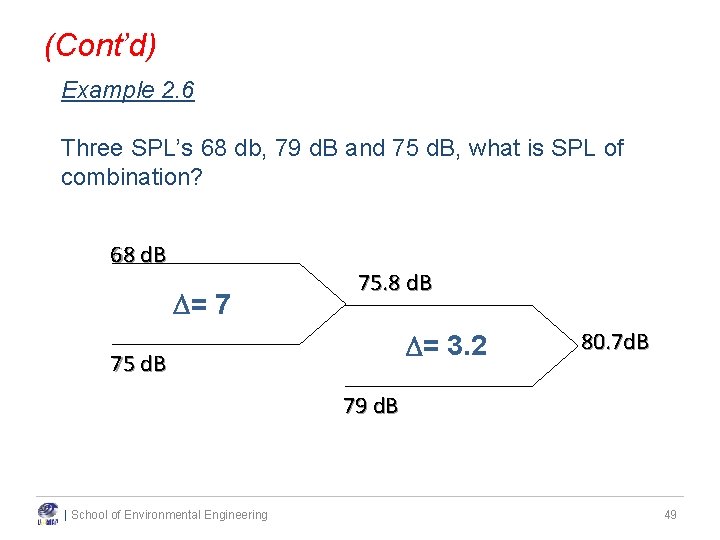
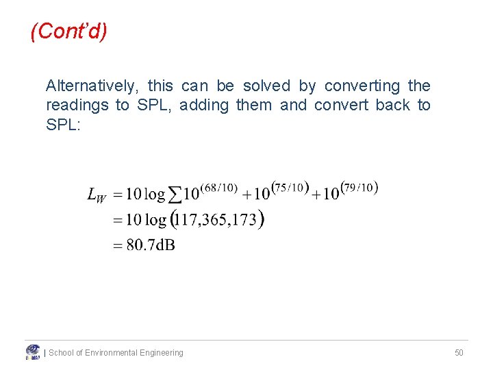
(Cont’d) Example 2. 6 Three SPL’s 68 db, 79 d. B and 75 d. B, what is SPL of combination? 68 d. B = 7 75. 8 d. B = 3. 2 75 d. B 80. 7 d. B 79 d. B | School of Environmental Engineering 49

(Cont’d) Alternatively, this can be solved by converting the readings to SPL, adding them and convert back to SPL: | School of Environmental Engineering 50

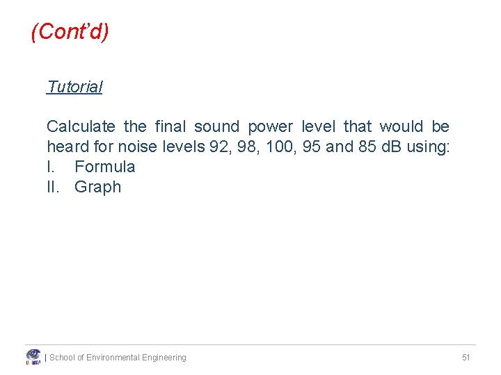
(Cont’d) Tutorial Calculate the final sound power level that would be heard for noise levels 92, 98, 100, 95 and 85 d. B using: I. Formula II. Graph | School of Environmental Engineering 51

| School of Environmental Engineering 52

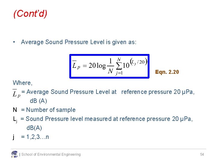
2. 2. 2. 6 Averaging Sound • Average sound can be calculated as the same as the calculation of summation of sound. • As sound is referred in form of log, so the average requires calculation in form of pressure and power. The pressure is then calculated, averaged and finally antilog. | School of Environmental Engineering 53

(Cont’d) • Average Sound Pressure Level is given as: Eqn. 2. 20 Where, = Average Sound Pressure Level at reference pressure 20 μPa, d. B (A) N = Number of sample Lj = Sound Pressure level measured at reference pressure 20 μPa, d. B(A) j = 1, 2, 3…n | School of Environmental Engineering 54

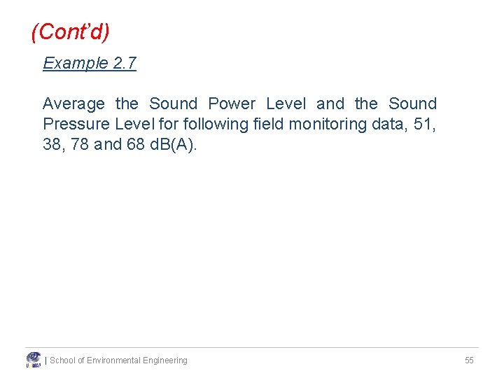
(Cont’d) Example 2. 7 Average the Sound Power Level and the Sound Pressure Level for following field monitoring data, 51, 38, 78 and 68 d. B(A). | School of Environmental Engineering 55

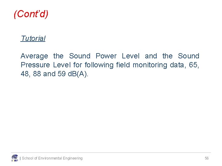
(Cont’d) Tutorial Average the Sound Power Level and the Sound Pressure Level for following field monitoring data, 65, 48, 88 and 59 d. B(A). | School of Environmental Engineering 56

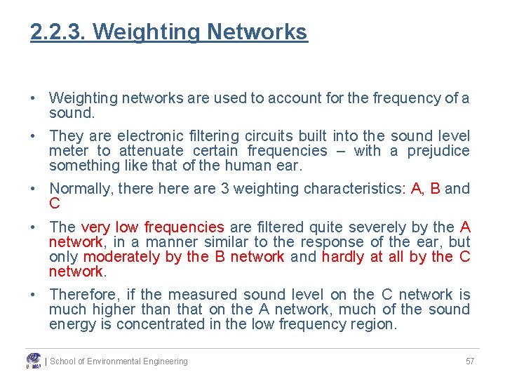
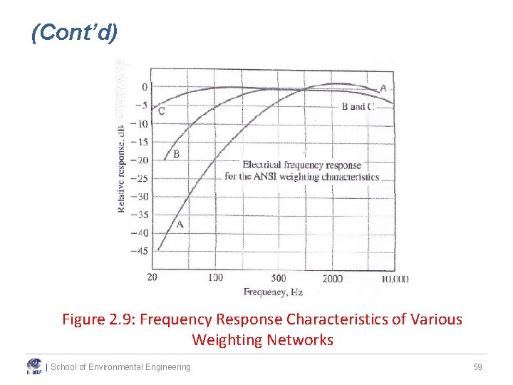
2. 2. 3. Weighting Networks • Weighting networks are used to account for the frequency of a sound. • They are electronic filtering circuits built into the sound level meter to attenuate certain frequencies – with a prejudice something like that of the human ear. • Normally, there are 3 weighting characteristics: A, B and C • The very low frequencies are filtered quite severely by the A network, in a manner similar to the response of the ear, but only moderately by the B network and hardly at all by the C network. • Therefore, if the measured sound level on the C network is much higher than that on the A network, much of the sound energy is concentrated in the low frequency region. | School of Environmental Engineering 57

(Cont’d) • “A” Scale – Filters out low frequencies – Response curve is similar to sensitivity of human ear • “C” Scale – Filters out very little (only the extreme low frequencies) – If a measurement is higher on the C scale than the A scale, the noise has a low frequency component – Used to estimate the effectiveness of ear protectors • A specialized filter, the "D" weighting, has also been introduced for aircraft noise measurements. • Figure 2. 9 shows the response characteristics of the three basic networks as prescribed by the American National Standards Institute (ANSI) spec. no. S 1. 4 – 1971. | School of Environmental Engineering 58

(Cont’d) Figure 2. 9: Frequency Response Characteristics of Various Weighting Networks | School of Environmental Engineering 59

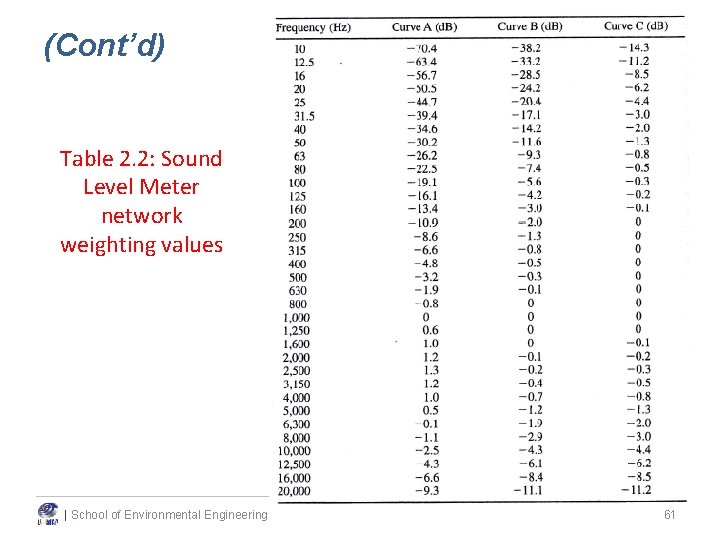
(Cont’d) • When a weighting network is used, the sound level meter is electronically subtracts or adds the number of d. B shown at each frequency shown in Table 2. 2 • Readings taken when a network is in use are said to be “sound levels” rather than “sound pressure levels”. • The readings taken are designated in decibels in one of the following forms: d. B(A), d. Ba, d. BA; d. B(B), d. Bb, d. BB; d. B(C), d. Bc, d. BC. Tabular notations may refer to LA , LB , LC | School of Environmental Engineering 60

(Cont’d) Table 2. 2: Sound Level Meter network weighting values | School of Environmental Engineering 61

(Cont’d) Example 2. 8 A new type 2 sound level meter is to be tested with two pure tone sources that emit 90 d. B. The two sources are at 1, 000 Hz and 100 Hz. Estimate the expected readings on the A, B and C weighting networks. | School of Environmental Engineering 62

(Cont’d) Example 2. 9 The following sound levels were measured on the A, B, and C weighting networks: Source 1: 94 d. B(A), 95 d. B(B) and 96 d. B(C) Source 2: 74 d. B(A), 83 d. B(B) and 90 d. B(C) Characterize the sources as “low frequency” or “mid/high frequency”. | School of Environmental Engineering 63

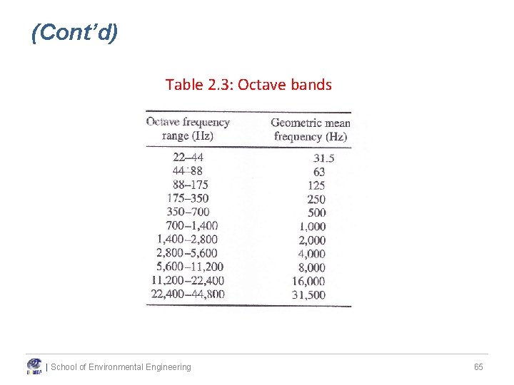
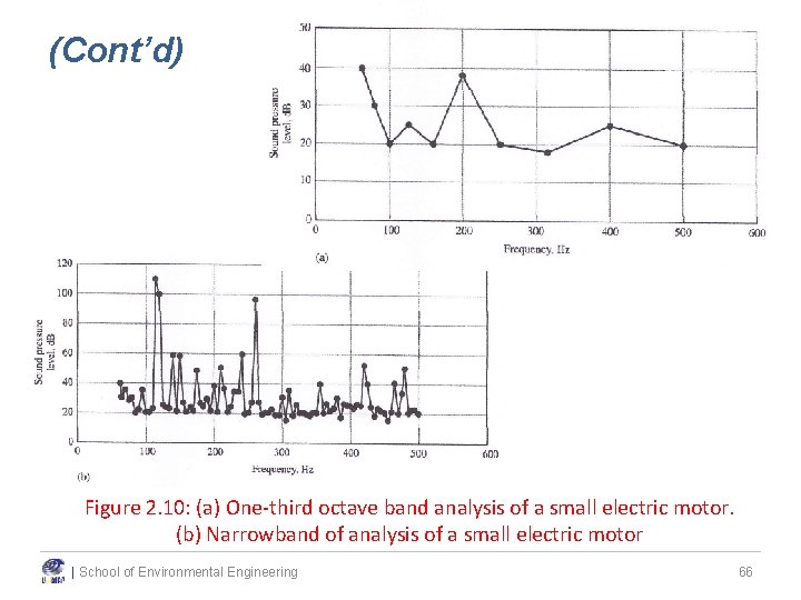
2. 2. 4. Octave Bands • To completely characterize a noise, it is necessary to break it down into its frequency components or spectra. • An octave is the frequency interval between a given frequency and twice the frequency • For example: given a 22 Hz frequency, so the octave band is from 22 to 44 Hz. A second octave band would be from 44 to 88 Hz. • Normally, considering an 8 to 11 octave bands • One third octave band analysis provides a slightly more refined picture of the noise source than the full octave band analysis | School of Environmental Engineering 64

(Cont’d) Table 2. 3: Octave bands | School of Environmental Engineering 65

(Cont’d) Figure 2. 10: (a) One-third octave band analysis of a small electric motor. (b) Narrowband of analysis of a small electric motor | School of Environmental Engineering 66

2. 2. 6. Rating Systems • Goals of Noise-Rating System – An ideal noise-rating system is one that allows measurements by sound level meters or analyzers to be summarized succinctly and yet represent noise exposure in a meaningful way – Our response to sound is strongly dependent on the frequency of the sound – Significant factors in annoyance: type of noise & time of day that it occurred – Ideal system: a) frequency, b) daytime or nighttime noise, c) capable of describing the cumulative noise exposure. | School of Environmental Engineering 67

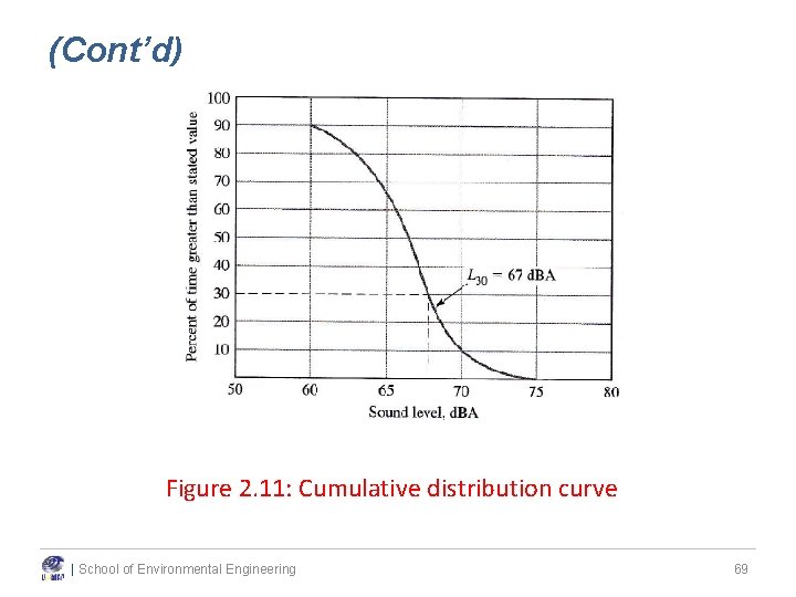
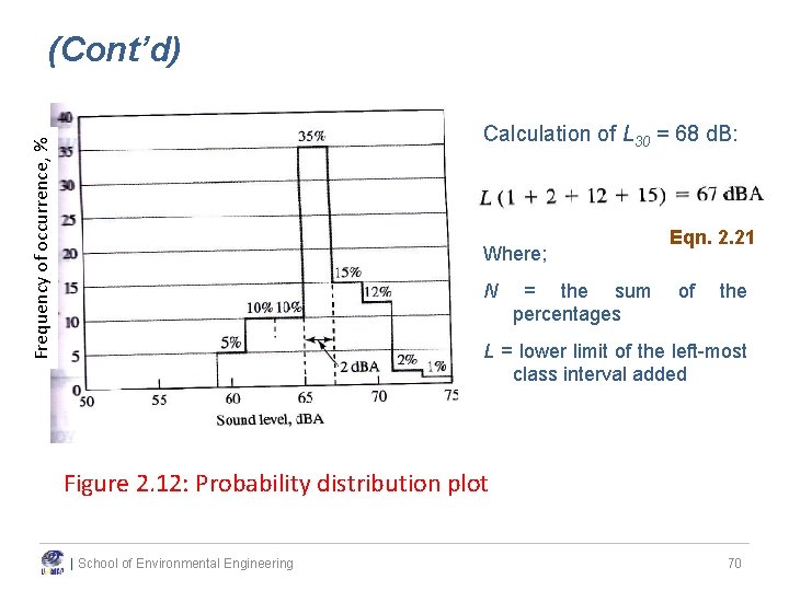
(Cont’d) The LN Concept • LN is a statistical measure that indicates how frequently a particular sound level is exceeded. • Example: if L 30 = 67 d. B, means that 67 d. B(A) was exceeded for 30% of the measuring time. • A plot of against N (where N = 1%, 2%, 3%, …. ) look like the cumulative distribution curve (Figure 2. 11) • Allied to the cumulative distribution curve is the probability distribution curve (Figure 2. 12) – showing how often the noise levels fall into certain class intervals. | School of Environmental Engineering 68

(Cont’d) Figure 2. 11: Cumulative distribution curve | School of Environmental Engineering 69

(Cont’d) Frequency of occurrence, % Calculation of L 30 = 68 d. B: Where; N = the sum percentages Eqn. 2. 21 of the L = lower limit of the left-most class interval added Figure 2. 12: Probability distribution plot | School of Environmental Engineering 70

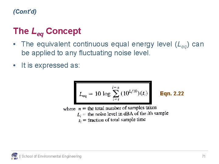
(Cont’d) The Leq Concept • The equivalent continuous equal energy level (Leq) can be applied to any fluctuating noise level. • It is expressed as: Eqn. 2. 22 | School of Environmental Engineering 71

(Cont’d) Example 2. 10 Consider the case where a noise level of 90 d. BA exists for 10 minutes and is followed by a reduced noise level of 70 d. BA for 30 minutes. What is the equivalent continuous equal energy level for the 40 minute period? Assume a five-minutes sampling interval. | School of Environmental Engineering 72

(Cont’d) The Ldn Concept • Ldn is the Leq computed over a 24 -hr period with a “penalty “ of 10 d. BA for a designated night time period. • Day-night average – subscript “dn” • In airport noise applications, Ldn is referred to LDN • Night time period 10 pm to 7 am • Ldn equation is derived from the Leq equation with the time increment specified as 1 s (1 86, 400 seconds) | School of Environmental Engineering 73

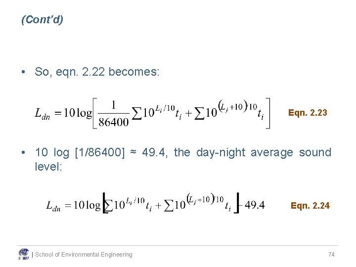
(Cont’d) • So, eqn. 2. 22 becomes: Eqn. 2. 23 • 10 log [1/86400] ≈ 49. 4, the day-night average sound level: Eqn. 2. 24 | School of Environmental Engineering 74

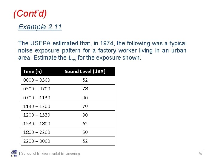
(Cont’d) Example 2. 11 The USEPA estimated that, in 1974, the following was a typical noise exposure pattern for a factory worker living in an urban area. Estimate the Ldn for the exposure shown. Time (h) Sound Level (d. BA) 0000 – 0500 52 0500 – 0700 78 0700 – 1130 90 1130 – 1200 70 1200 – 1530 90 1530 – 1800 52 1800 – 2200 60 2200 – 0000 52 | School of Environmental Engineering 75

d n t u n o e S ) m 3 e 2. sur ea M | School of Environmental Engineering 76

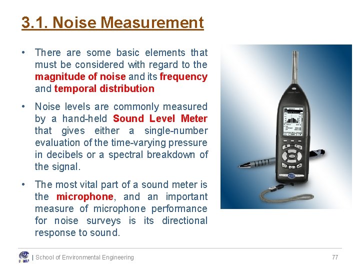
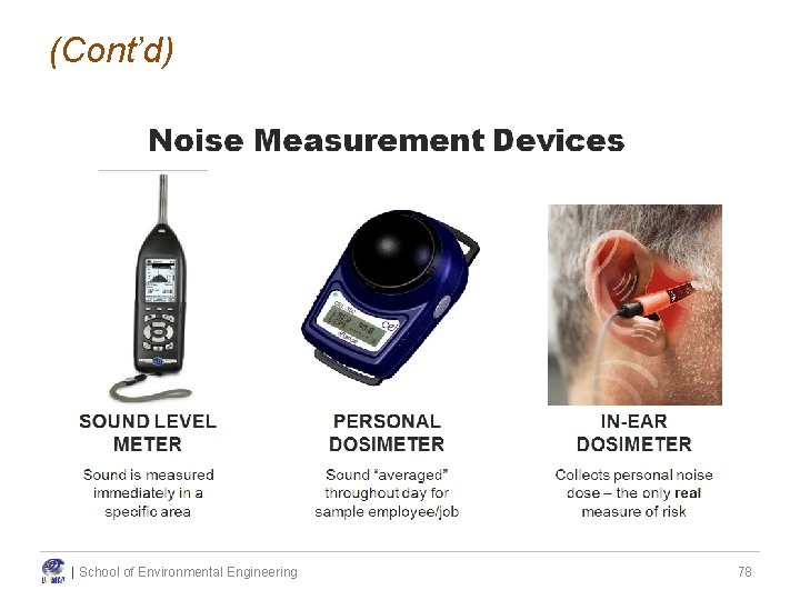
3. 1. Noise Measurement • There are some basic elements that must be considered with regard to the magnitude of noise and its frequency and temporal distribution • Noise levels are commonly measured by a hand-held Sound Level Meter that gives either a single-number evaluation of the time-varying pressure in decibels or a spectral breakdown of the signal. • The most vital part of a sound meter is the microphone, and an important measure of microphone performance for noise surveys is its directional response to sound. | School of Environmental Engineering 77

(Cont’d) | School of Environmental Engineering 78

(Cont’d) • An integrating Sound Level Meter monitoring which was capable of readout of the noise level readings continuous sound pressure level (Lx). was used for noise giving a continuous including equivalent (Leq) and percentile • Sound Level Meter shall be installed in flat terrain having no excessive sound absorption characteristics such as thick, matted or tall grasses, shrubs, or wooded areas. No obstructions significantly influencing the sound field from the sources shall exist within a conical space above the point on the ground vertically below the microphone. • The microphone height shall be at least 4 m, preferably 10 m, above the ground level. | School of Environmental Engineering 79

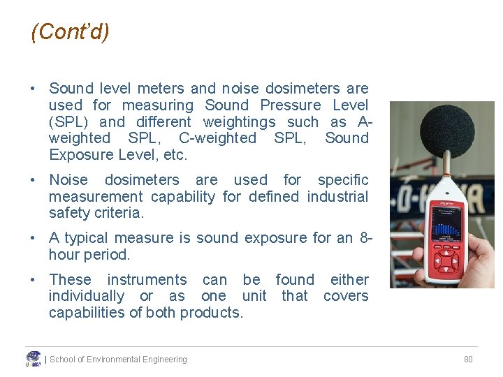
(Cont’d) • Sound level meters and noise dosimeters are used for measuring Sound Pressure Level (SPL) and different weightings such as Aweighted SPL, C-weighted SPL, Sound Exposure Level, etc. • Noise dosimeters are used for specific measurement capability for defined industrial safety criteria. • A typical measure is sound exposure for an 8 hour period. • These instruments can be found either individually or as one unit that covers capabilities of both products. | School of Environmental Engineering 80

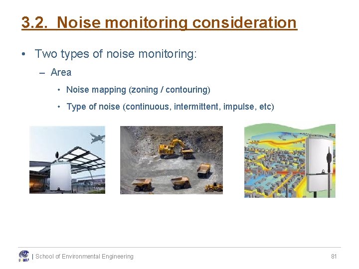
3. 2. Noise monitoring consideration • Two types of noise monitoring: – Area • Noise mapping (zoning / contouring) • Type of noise (continuous, intermittent, impulse, etc) | School of Environmental Engineering 81

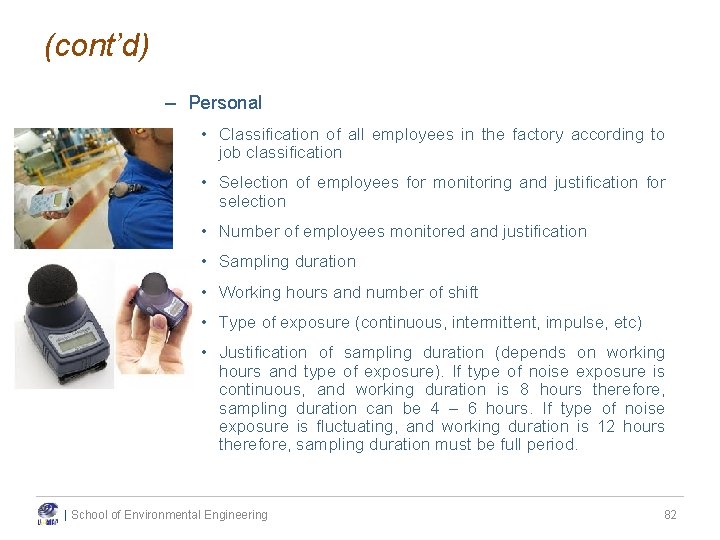
(cont’d) – Personal • Classification of all employees in the factory according to job classification • Selection of employees for monitoring and justification for selection • Number of employees monitored and justification • Sampling duration • Working hours and number of shift • Type of exposure (continuous, intermittent, impulse, etc) • Justification of sampling duration (depends on working hours and type of exposure). If type of noise exposure is continuous, and working duration is 8 hours therefore, sampling duration can be 4 – 6 hours. If type of noise exposure is fluctuating, and working duration is 12 hours therefore, sampling duration must be full period. | School of Environmental Engineering 82

| School of Environmental Engineering 83