Sampling Technical Aspects Sampling Have discussed different types

Sampling Technical Aspects

Sampling • Have discussed different types of sampling – Quota, convenience, judgement and probability samples • Will now focus on probability sampling – Theoretical framework – Various probability sampling concepts • Stratification, clustering, unequal selection probabilities • Systematic sampling; multi-stage sampling

Simple Random Samples • Say we decide to take a sample of size n • If all the possible samples have an equal probability of being chosen, this is called a simple random sample (without replacement), or SRS for short • Can also take a simple random sample with replacement (SRSWR), but this requires a slightly more general sampling theory

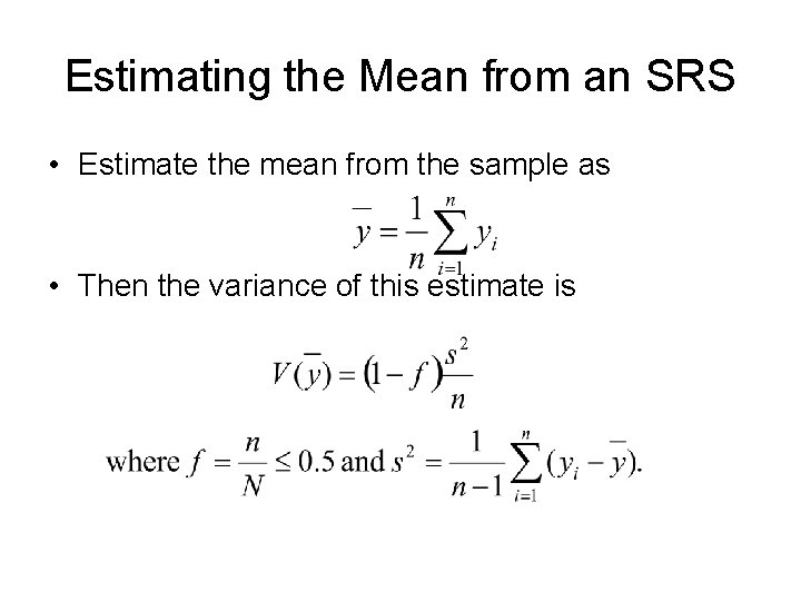
Estimating the Mean from an SRS • Estimate the mean from the sample as • Then the variance of this estimate is

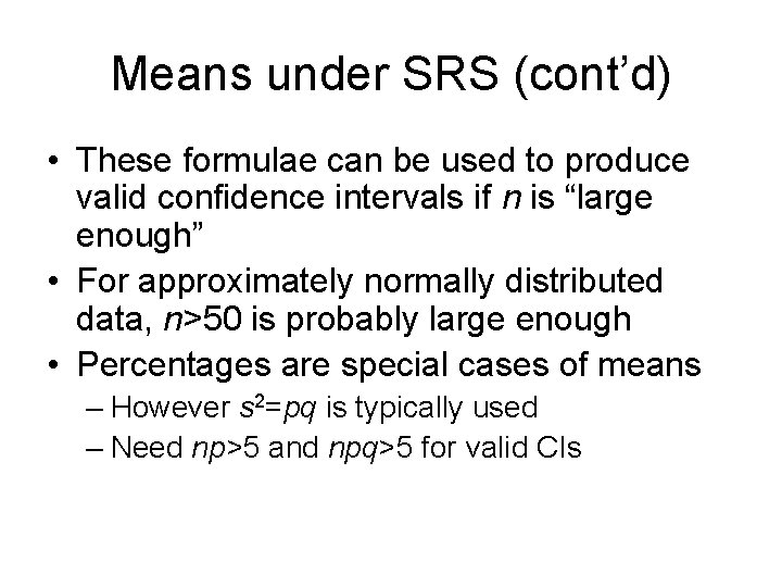
Means under SRS (cont’d) • These formulae can be used to produce valid confidence intervals if n is “large enough” • For approximately normally distributed data, n>50 is probably large enough • Percentages are special cases of means – However s 2=pq is typically used – Need np>5 and npq>5 for valid CIs

Other Sample Designs • SRS are often too costly for practical use • Other sample designs are therefore needed • Stratified sampling – Split population into groups or strata – Sample independently within each stratum – Can use different sampling fractions within each stratum (or even various sample designs)

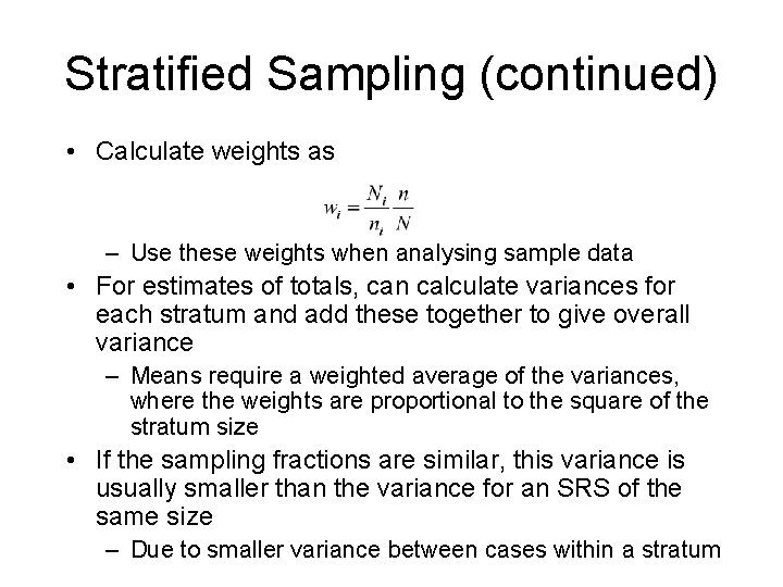
Stratified Sampling (continued) • Calculate weights as – Use these weights when analysing sample data • For estimates of totals, can calculate variances for each stratum and add these together to give overall variance – Means require a weighted average of the variances, where the weights are proportional to the square of the stratum size • If the sampling fractions are similar, this variance is usually smaller than the variance for an SRS of the same size – Due to smaller variance between cases within a stratum

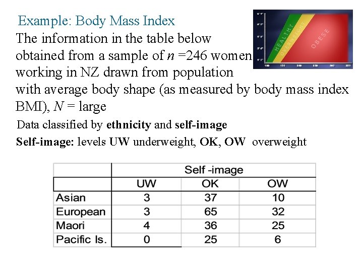
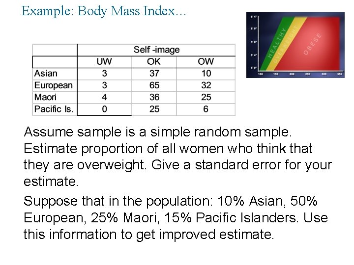
Example: Body Mass Index The information in the table below obtained from a sample of n =246 women working in NZ drawn from population with average body shape (as measured by body mass index BMI), N = large Data classified by ethnicity and self-image Self-image: levels UW underweight, OK, OW overweight

Example: Body Mass Index… Assume sample is a simple random sample. Estimate proportion of all women who think that they are overweight. Give a standard error for your estimate. Suppose that in the population: 10% Asian, 50% European, 25% Maori, 15% Pacific Islanders. Use this information to get improved estimate.

Cluster Sampling • Typically, face-to-face household surveys involve interviewing several people in each area • This is an example of a cluster sample, where the areas are the clusters • This approach is much less costly than an SRS of the same size • However it will also exhibit higher sampling variability, due to correlations between interviews within a cluster – E. g. similar spending patterns due to similar incomes, or a similar range of products being available locally

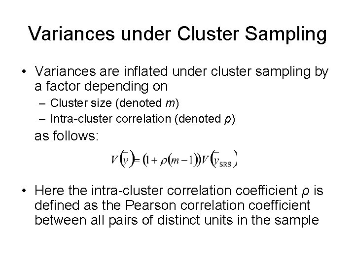
Variances under Cluster Sampling • Variances are inflated under cluster sampling by a factor depending on – Cluster size (denoted m) – Intra-cluster correlation (denoted ρ) as follows: • Here the intra-cluster correlation coefficient ρ is defined as the Pearson correlation coefficient between all pairs of distinct units in the sample

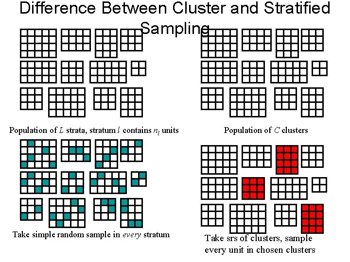
Difference Between Cluster and Stratified Sampling Population of L strata, stratum l contains nl units Take simple random sample in every stratum Population of C clusters Take srs of clusters, sample every unit in chosen clusters

Systematic Sampling • Another commonly used sampling technique is systematic sampling • The population is listed in a particular order, then every kth unit is selected – Start at a random point between 1 and k – Here k is chosen so that N ≈ kn • Systematic sampling is a special case of cluster sampling, with only one cluster selected – This makes it hard to estimate sampling variances • Need prior knowledge or assumptions about response patterns

More on Systematic Sampling • Performance depends strongly on response patterns – Linear trend yields an implicit stratification, and works well – However cyclic variation of period k (or some multiple of k) can result in huge variability • Systematic sampling generalises easily to sampling with probability proportional to size – However large units may need to be placed in a certainty stratum, or selected more than once

Multi-stage Sample Designs • Many surveys use complex sample designs that combine several of the above elements in a multi -stage sampling framework • For example, face-to-face in-home surveys of people often employ three stages – Systematic pps sampling of areas – Cluster samples of households within areas – Random selection of one person from each household (unequal sampling probabilities)

Complex Sample Designs • Multi-stage designs may require complex estimation processes, especially for variance estimation – Specialised software is often needed • Different items in a questionnaire may refer to different units, from different sampling stages – E. g. Households and people – E. g. Customers and brands purchased – These will usually require different statistical treatment • E. g. different sets of weights for households and people

After you’ve collected the data

Data Collection • Contact selected respondents – Unless data can be obtained ethically through observation or record linkage/data matching • Obtain completed questionnaires – Structured interview or self-completion • Statistics involved here in design decisions – E. g. quotas, scheduling interview times • Also quality control and improvement role

Data Capture and Cleaning • Data entry – From paper questionnaires or other records – Typically a (fixed) proportion are re-entered for quality control (QC) purposes – improvement possible here • Coding – Assigning labels (or codes) based on verbal descriptions • Data editing – Eliminate inconsistent data – Identify and treat outliers • Confirm data with respondent, or alter or even delete data

Weighting and Imputation • Weighting – Attaches a weight to each observation – Used to calculate weighted means, percentages – Often required to reflect sample design • Un-weighted results would be biased – Also helps compensate for unit non-response • Unit non-response is when data is not obtained for some units, although they were selected as part of our sample • Weights are adjusted to align survey results with known population figures – Covered in more detail later

Imputation • Helps deal with item missing data – When certain items in the questionnaire are not available for all respondents, this is known as item missing data • Fills in gaps with sensible values • Allows standard methods for analysis of complete data to be used • More detail given later

Data Analysis and Tables • Many analysis techniques are available • Cross-tabulation is ubiquitous in market research – Tabulating one categorical variable against another, e. g. intended party vote by age group • Need to calculate random sampling error – Also known as variance estimation – Influenced by sample design and weighting – More on this later

Reporting and Decision-Making • Reporting results – Important that these are communicated clearly • Statistical input often vital – Should address survey objectives • Decision-making and action – Influenced by survey results (hopefully!) – Actions may include further research

Statistics in Survey Research • In summary: – Statistics is generally most useful in the design and analysis stages of surveys • Especially sampling, weighting, and data analysis – Also relevant at other stages • Quality control and quality improvement for survey operations • Effect of survey procedures on survey results • Interpretation of survey results

Weighting • Usually survey weights are calculated for each responding unit • Aim for unbiased weighted survey results – Or at least more accurate than without weights • Survey weights can adjust for – Sample design – Unit non-response

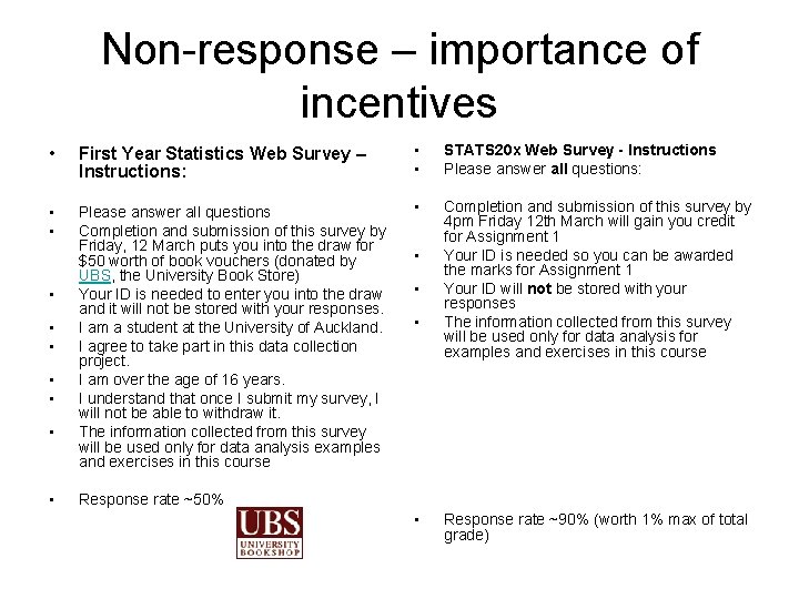
Non-response – importance of incentives • First Year Statistics Web Survey – Instructions: • • STATS 20 x Web Survey - Instructions Please answer all questions: • • Please answer all questions Completion and submission of this survey by Friday, 12 March puts you into the draw for $50 worth of book vouchers (donated by UBS, the University Book Store) Your ID is needed to enter you into the draw and it will not be stored with your responses. I am a student at the University of Auckland. I agree to take part in this data collection project. I am over the age of 16 years. I understand that once I submit my survey, I will not be able to withdraw it. The information collected from this survey will be used only for data analysis examples and exercises in this course • Completion and submission of this survey by 4 pm Friday 12 th March will gain you credit for Assignment 1 Your ID is needed so you can be awarded the marks for Assignment 1 Your ID will not be stored with your responses The information collected from this survey will be used only for data analysis for examples and exercises in this course • • • Response rate ~50% • Response rate ~90% (worth 1% max of total grade)

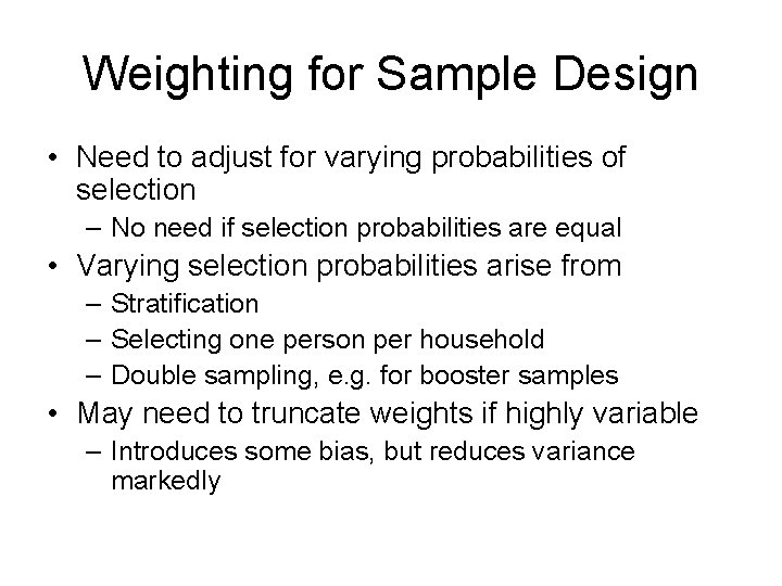
Weighting for Sample Design • Need to adjust for varying probabilities of selection – No need if selection probabilities are equal • Varying selection probabilities arise from – Stratification – Selecting one person per household – Double sampling, e. g. for booster samples • May need to truncate weights if highly variable – Introduces some bias, but reduces variance markedly

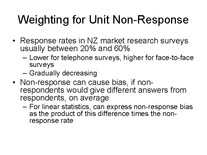
Weighting for Unit Non-Response • Response rates in NZ market research surveys usually between 20% and 60% – Lower for telephone surveys, higher for face-to-face surveys – Gradually decreasing • Non-response can cause bias, if nonrespondents would give different answers from respondents, on average – For linear statistics, can express non-response bias as the product of this difference times the nonresponse rate

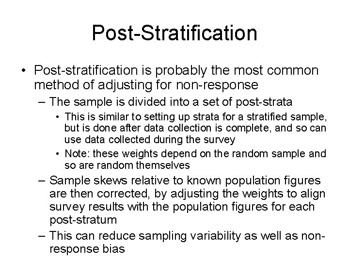
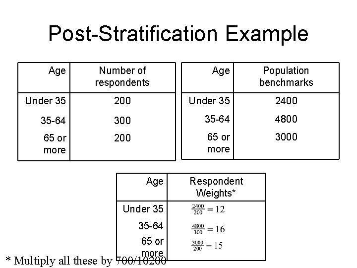
Post-Stratification • Post-stratification is probably the most common method of adjusting for non-response – The sample is divided into a set of post-strata • This is similar to setting up strata for a stratified sample, but is done after data collection is complete, and so can use data collected during the survey • Note: these weights depend on the random sample and so are random themselves – Sample skews relative to known population figures are then corrected, by adjusting the weights to align survey results with the population figures for each post-stratum – This can reduce sampling variability as well as nonresponse bias

Post-Stratification Example Age Number of respondents Age Population benchmarks Under 35 200 Under 35 2400 35 -64 300 35 -64 4800 65 or more 200 65 or more 3000 Age Under 35 35 -64 65 or more * Multiply all these by 700/10200 Respondent Weights*

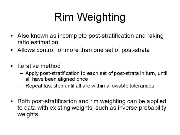
Rim Weighting • Also known as incomplete post-stratification and raking ratio estimation • Allows control for more than one set of post-strata • Iterative method – Apply post-stratification to each set of post-strata in turn, until all have been aligned once – Repeat last step until all are within allowable tolerances • Both post-stratification and rim weighting can be applied to data with existing weights, such as inverse probability weights

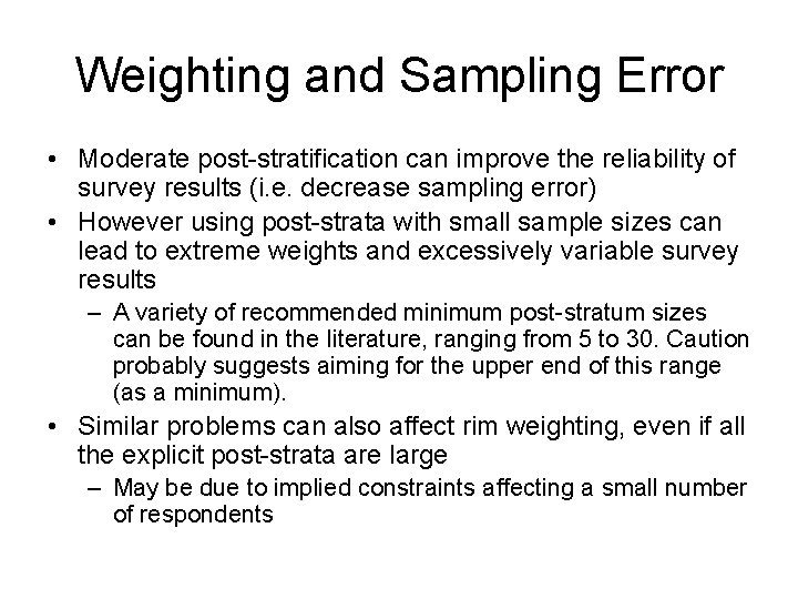
Weighting and Sampling Error • Moderate post-stratification can improve the reliability of survey results (i. e. decrease sampling error) • However using post-strata with small sample sizes can lead to extreme weights and excessively variable survey results – A variety of recommended minimum post-stratum sizes can be found in the literature, ranging from 5 to 30. Caution probably suggests aiming for the upper end of this range (as a minimum). • Similar problems can also affect rim weighting, even if all the explicit post-strata are large – May be due to implied constraints affecting a small number of respondents

Data checking and Imputation

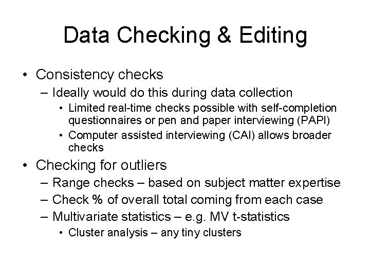
Data Checking & Editing • Consistency checks – Ideally would do this during data collection • Limited real-time checks possible with self-completion questionnaires or pen and paper interviewing (PAPI) • Computer assisted interviewing (CAI) allows broader checks • Checking for outliers – Range checks – based on subject matter expertise – Check % of overall total coming from each case – Multivariate statistics – e. g. MV t-statistics • Cluster analysis – any tiny clusters

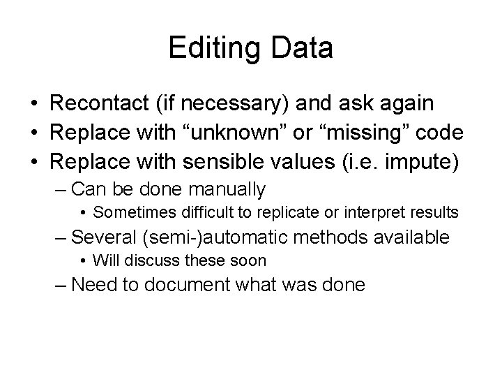
Editing Data • Recontact (if necessary) and ask again • Replace with “unknown” or “missing” code • Replace with sensible values (i. e. impute) – Can be done manually • Sometimes difficult to replicate or interpret results – Several (semi-)automatic methods available • Will discuss these soon – Need to document what was done

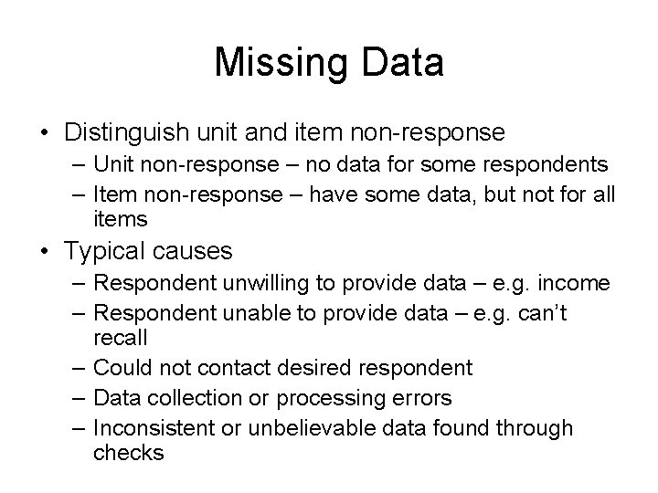
Missing Data • Distinguish unit and item non-response – Unit non-response – no data for some respondents – Item non-response – have some data, but not for all items • Typical causes – Respondent unwilling to provide data – e. g. income – Respondent unable to provide data – e. g. can’t recall – Could not contact desired respondent – Data collection or processing errors – Inconsistent or unbelievable data found through checks

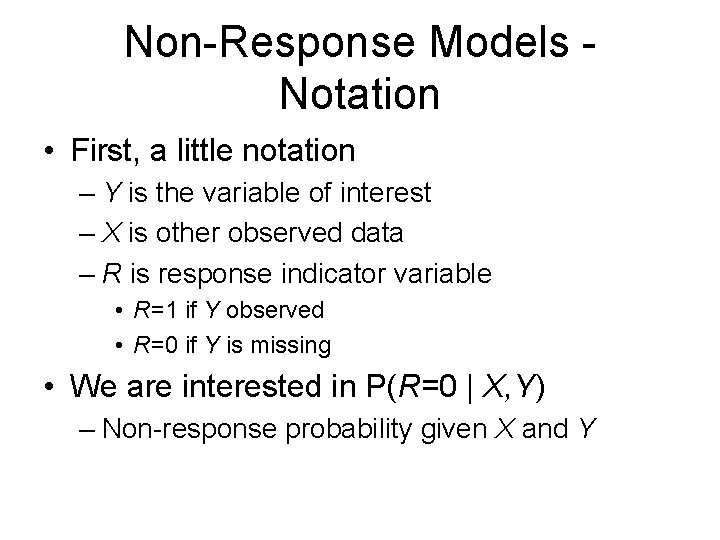
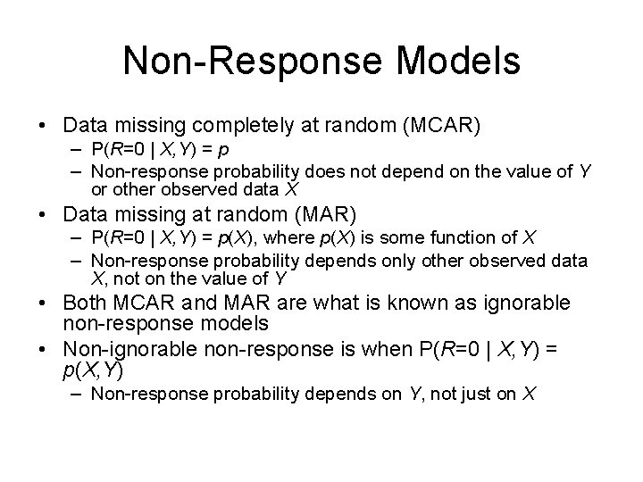
Non-Response Models Notation • First, a little notation – Y is the variable of interest – X is other observed data – R is response indicator variable • R=1 if Y observed • R=0 if Y is missing • We are interested in P(R=0 | X, Y) – Non-response probability given X and Y

Non-Response Models • Data missing completely at random (MCAR) – P(R=0 | X, Y) = p – Non-response probability does not depend on the value of Y or other observed data X • Data missing at random (MAR) – P(R=0 | X, Y) = p(X), where p(X) is some function of X – Non-response probability depends only other observed data X, not on the value of Y • Both MCAR and MAR are what is known as ignorable non-response models • Non-ignorable non-response is when P(R=0 | X, Y) = p(X, Y) – Non-response probability depends on Y, not just on X

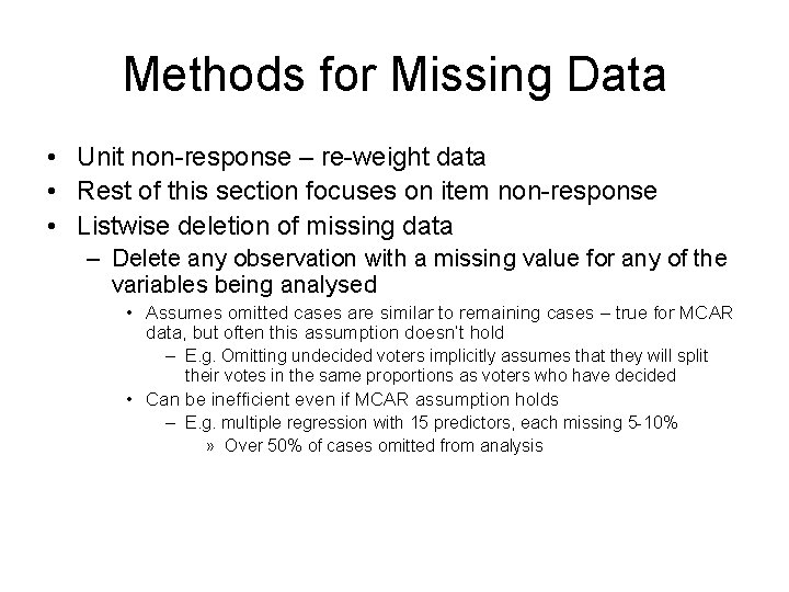
Methods for Missing Data • Unit non-response – re-weight data • Rest of this section focuses on item non-response • Listwise deletion of missing data – Delete any observation with a missing value for any of the variables being analysed • Assumes omitted cases are similar to remaining cases – true for MCAR data, but often this assumption doesn’t hold – E. g. Omitting undecided voters implicitly assumes that they will split their votes in the same proportions as voters who have decided • Can be inefficient even if MCAR assumption holds – E. g. multiple regression with 15 predictors, each missing 5 -10% » Over 50% of cases omitted from analysis

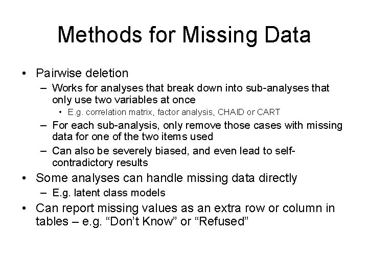
Methods for Missing Data • Pairwise deletion – Works for analyses that break down into sub-analyses that only use two variables at once • E. g. correlation matrix, factor analysis, CHAID or CART – For each sub-analysis, only remove those cases with missing data for one of the two items used – Can also be severely biased, and even lead to selfcontradictory results • Some analyses can handle missing data directly – E. g. latent class models • Can report missing values as an extra row or column in tables – e. g. “Don’t Know” or “Refused”

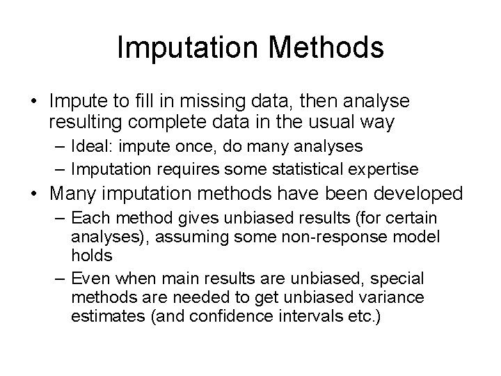
Imputation Methods • Impute to fill in missing data, then analyse resulting complete data in the usual way – Ideal: impute once, do many analyses – Imputation requires some statistical expertise • Many imputation methods have been developed – Each method gives unbiased results (for certain analyses), assuming some non-response model holds – Even when main results are unbiased, special methods are needed to get unbiased variance estimates (and confidence intervals etc. )

Mean Imputation • Mean imputation – Impute mean value for all missing values – Gives sensible overall mean (assuming data MCAR), but distorts distribution • Impute mean + simulated error • Impute mean + random residual • Impute mean within imputation classes – Only assumes data MAR (where X=imputation class) when estimating means – Can generalise all the above methods to incorporate ANOVA or regression models

Hot-deck Imputation • Random hot-deck imputation – Divide data into imputation classes – Replace each missing value with the data from a randomly chosen donor in the same class – Assumes MAR (where X=imputation class) – Preserves distribution within classes – However only works well for moderately large imputation classes (preferably 30+, depends on nature of Y distribution given X) • Also multivariate (X, Y) relationships are hard to handle

Hot-deck Imputation • Nearest neighbour hot-deck imputation – Choose from most similar donors available, based on a multivariate distance function • Can choose best match, or randomly from k best • Can limit donor usage by including penalty for heavy usage into distance function – Allows for multivariate (X, Y) relationships – Not limited to a specific statistical model • Can be less efficient than methods that do assume a specific model, but is more robust

Multiple Imputation • Aims to allow valid inference when certain imputation methods are used (Rubin 1987) • Method – Impute multiple values using same imputation procedure – Analyse each resulting dataset, recording results including variance estimates – Combine the results to give overall variance estimate, and use this for inference

Multiple Imputation • Whether this works depends on the data, the analysis being carried out and the imputation method used • When it works, the imputation method is called “proper” (for that analysis procedure and dataset) • However it is difficult to know whether it works for a particular analysis • Current advice is to use a wide selection of X variables when imputing, including all possible analysis variables and design factors • Other methods have been developed for correct imputation inference – more details later

Variance estimation

Variance Estimation • Sampling variation depends on the estimator, sample design and sample size – Many market researchers believe it depends only on sample size – e. g. net percentages • Standard variance formulae available for most analysis methods – Typically assume SRS or SRSWR • However these formulae do not work for the sample designs used in most MR surveys

Classical Approaches • Variance formulae have also been developed for some estimators under a wide range of sample designs – See books by authors such as Cochran and Kish • 1950’s to 1970’s • Design effect – Ratio of actual variance to variance assuming SRS of same size – Typically varies from one item to the next • Usually under 2 for household surveys, but sometimes more • Can be much higher for other surveys – e. g. 25 for some items in NZ Adverse Events Study

General Methods for Variance Estimation • Variance formulae may already be available • If not, there are several general methods for variance estimation for complex surveys – Linearisation – Random groups – Resampling methods • Balanced repeated replication (BRR) • Jackknife

Linearisation • Derives variances for non-linear statistics from variances (and covariances) for means or totals • Use Taylor’s theorem to approximate around the estimate by a linear function – See Lohr (1999) formulae and examples • Widely used; common analyses are implemented for many designs in software such as SUDAAN • Only works for smooth functions of totals – E. g. not for medians or other quantiles • Also difficult to apply for complex weights • Can produce variances that are too small for small samples

Random Groups • Original idea (Mahalonobis 1946) – Select several independent samples using the sample design: “interpenetrating samples” – Calculate survey results for each sample or replicate – Use variation between the results from each of these samples to estimate the variance • Not usually practical to draw enough separate samples – Need >=10 samples to get accurate variance estimates • Instead, draw one sample and divide it into groups with each being a miniature version of the whole

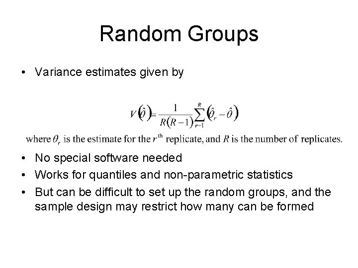
Random Groups • Variance estimates given by • No special software needed • Works for quantiles and non-parametric statistics • But can be difficult to set up the random groups, and the sample design may restrict how many can be formed

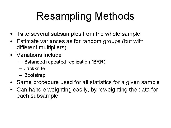
Resampling Methods • Take several subsamples from the whole sample • Estimate variances as for random groups (but with different multipliers) • Variations include – Balanced repeated replication (BRR) – Jackknife – Bootstrap • Same procedure used for all statistics for a given sample • Can handle weighting easily, by reweighting the data for each subsample

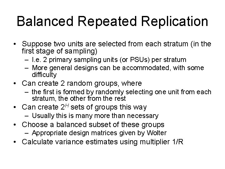
Balanced Repeated Replication • Suppose two units are selected from each stratum (in the first stage of sampling) – I. e. 2 primary sampling units (or PSUs) per stratum – More general designs can be accommodated, with some difficulty • Can create 2 random groups, where – the first is formed by randomly selecting one unit from each stratum, the other from the rest • Can create 2 H sets of groups this way – Usually this is many more than necessary • Choose a balanced subset of these groups – Appropriate design matrices given by Wolter • Calculate variance estimates using multiplier 1/R

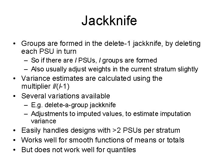
Jackknife • Groups are formed in the delete-1 jackknife, by deleting each PSU in turn – So if there are l PSUs, l groups are formed – Also usually adjust weights in the current stratum slightly • Variance estimates are calculated using the multiplier l/(l-1) • Several variations available – E. g. delete-a-group jackknife – Adjustments to imputed values, to estimate imputation variance • Easily handles designs with >2 PSUs per stratum • Works well for smooth functions of means or totals • But does not work well for quantiles

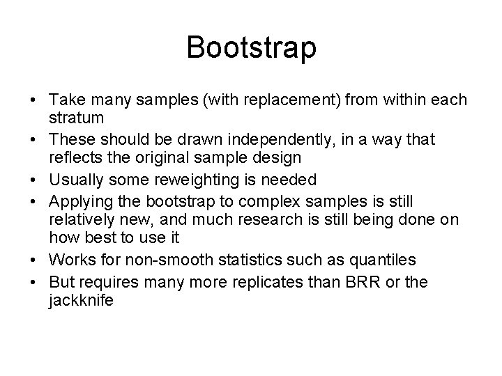
Bootstrap • Take many samples (with replacement) from within each stratum • These should be drawn independently, in a way that reflects the original sample design • Usually some reweighting is needed • Applying the bootstrap to complex samples is still relatively new, and much research is still being done on how best to use it • Works for non-smooth statistics such as quantiles • But requires many more replicates than BRR or the jackknife

Variance Estimation Software • SUDAAN – mainly uses linearisation methods • WESVAR – mainly uses BRR and the jackknife • SAS –now handles some common statistics and sample designs, using linearisation methods • VPLX – free software, based on replication approaches (primarily the jackknife) • Several other packages available – See http: //www. fas. harvard. edu/~stats/surveysoft/survey-soft. html for details

Variance Estimation - Summary • Important to realise that sample design affects sampling variation • Many methods to calculate correct sampling errors • Have given a quick overview here • Off-the-shelf software can handle some common situations • More complex estimators or weighting methods, or situations involving imputation, will usually require customised approach • Be careful – this can be quite a technical area – Easy to make significant mistakes – Best to get good advice when beginning to plan the survey if variance estimation is needed (i. e. at the sample design stage)