Sampling Design Avoiding Pitfalls in Environmental Sampling Part

Sampling Design Avoiding Pitfalls in Environmental Sampling Part 2 1

U. S. EPA Technical Session Agenda u Welcome u Understanding: Where does decision uncertainty come from? u Criteria: You can’t find the answer if you don’t know the question! u Pitfalls: How to lie (or at least be completely wrong) with statistics… u Solution Options: Truth serum for environmental decision-making 2

Solution Options: Truth serum for environmental decision-making “All truths are easy to understand once they are discovered; the point is to discover them. ” Galileo 9/15/2020 3

Triad Data Collection Design and Analysis Built On: u Planning systematically (Conceptual Site Models [CSM]) u Improving representativeness u Increasing information available for decision- making via real-time methods u Addressing the unknown with dynamic work strategies 4

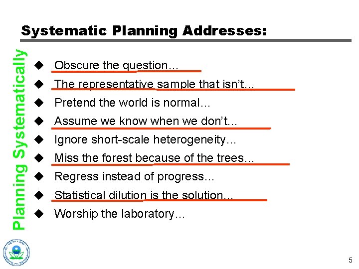
Planning Systematically Systematic Planning Addresses: u Obscure the question… u The representative sample that isn’t… u Pretend the world is normal… u Assume we know when we don’t… u Ignore short-scale heterogeneity… u Miss the forest because of the trees… u Regress instead of progress… u Statistical dilution is the solution… u Worship the laboratory… 5

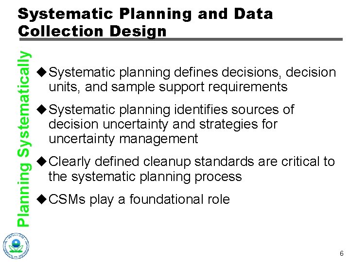
Planning Systematically Systematic Planning and Data Collection Design u Systematic planning defines decisions, decision units, and sample support requirements u Systematic planning identifies sources of decision uncertainty and strategies for uncertainty management u Clearly defined cleanup standards are critical to the systematic planning process u CSMs play a foundational role 6

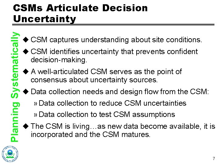
Planning Systematically CSMs Articulate Decision Uncertainty u CSM captures understanding about site conditions. u CSM identifies uncertainty that prevents confident decision-making. u A well-articulated CSM serves as the point of consensus about uncertainty sources. u Data collection needs and design flow from the CSM: » Data collection to reduce CSM uncertainties » Data collection to test CSM assumptions u The CSM is living…as new data become available, it is incorporated and the CSM matures. 7

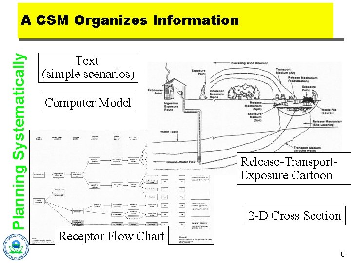
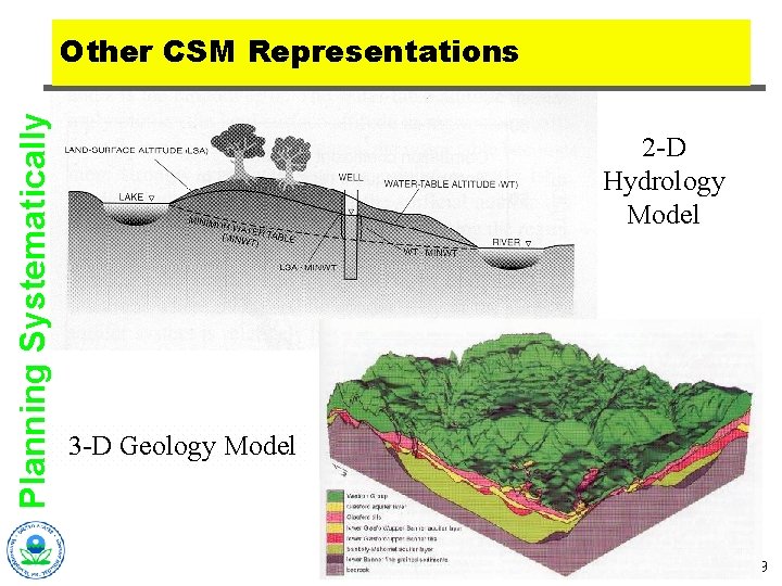
Planning Systematically A CSM Organizes Information Text (simple scenarios) Computer Model Release-Transport. Exposure Cartoon 2 -D Cross Section Receptor Flow Chart 8

Planning Systematically Other CSM Representations 2 -D Hydrology Model 3 -D Geology Model 9

Improving Representativeness Improving Data Representativeness Addresses: u Obscure the question… u The representative sample that isn’t… u Pretend the world is normal… u Assume we know when we don’t… u Ignore short-scale heterogeneity… u Miss the forest because of the trees… u Regress instead of progress… u Statistical dilution is the solution… u Worship the laboratory… 10

Improving Representativeness Improving Data Representativeness u Sample support » Matching sample support with decision needs » Field of view for in situ analyses u Controlling within-sample heterogeneity » Appropriate sample preparation important (see EPA/600/R-03/027 for additional detail) » Uncertainty effects quantified by appropriate subsample replicate analyses u Controlling short-scale heterogeneity » Multi-increment sampling » Aggregating in situ measurements 11

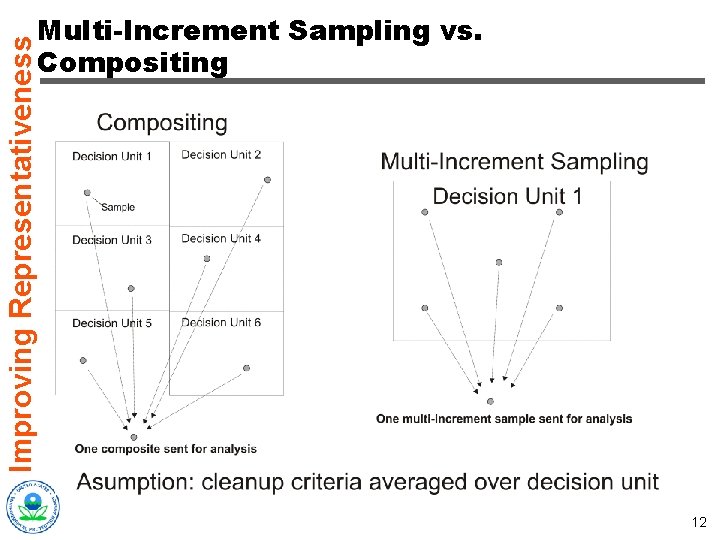
Improving Representativeness Multi-Increment Sampling vs. Compositing 12

Improving Representativeness Multi-Increment Sampling vs. Compositing u Multi-increment sampling: a strategy to control the effects of heterogeneity costeffectively u Compositing: a strategy to reduce overall analytical costs when conditions are favorable 13

Improving Representativeness Multi-Increment Sampling u Used to cost-effectively suppress short-scale heterogeneity u Multiple sub-samples contribute to sample that is analyzed u Sub-samples systematically distributed over an area equivalent to or less than decision requirements u Effective when the cost of analysis is significantly greater than the cost of sample acquisition 14

Improving Representativeness How Many Increments? u Enough to bring short-scale heterogeneity under control relative to other sources of error u Practical upper limit imposed by homogenization capacity u Level of heterogeneity present best estimated with a real-time technique » At least 10 measurements to get an estimate of variability at contaminant level of interest » Variability estimate can be used to determine how many increments should be used 15

Increasing Information via Real Time Methods u Obscure the question… u The representative sample that isn’t… u Pretend the world is normal… u Assume we know when we don’t… u Ignore short-scale heterogeneity… u Miss the forest because of the trees… u Regress instead of progress… u Statistical dilution is the solution… u Worship the laboratory… 16

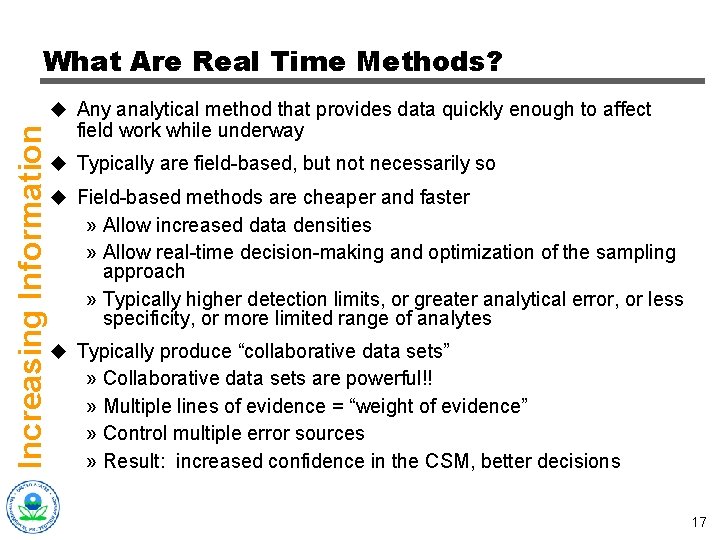
What Are Real Time Methods? Increasing Information u Any analytical method that provides data quickly enough to affect field work while underway u Typically are field-based, but not necessarily so u Field-based methods are cheaper and faster » Allow increased data densities » Allow real-time decision-making and optimization of the sampling approach » Typically higher detection limits, or greater analytical error, or less specificity, or more limited range of analytes u Typically produce “collaborative data sets” » Collaborative data sets are powerful!! » Multiple lines of evidence = “weight of evidence” » Control multiple error sources » Result: increased confidence in the CSM, better decisions 17

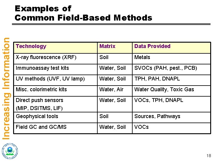
Increasing Information Examples of Common Field-Based Methods Technology Matrix Data Provided X-ray fluorescence (XRF) Soil Metals Immunoassay test kits Water, Soil SVOCs (PAH, pest. , PCB) UV methods (UVF, UV lamp) Water, Soil TPH, PAH, DNAPL Misc. colorimetric kits Water, Air Water Quality, Toxic Gas Direct push sensors Water, Soil VOCs, TPH, DNAPL (MIP, DSITMS, LIF) Geophysical tools Soil Sources, Pathways Field GC and GC/MS Water, Soil VOCs 18

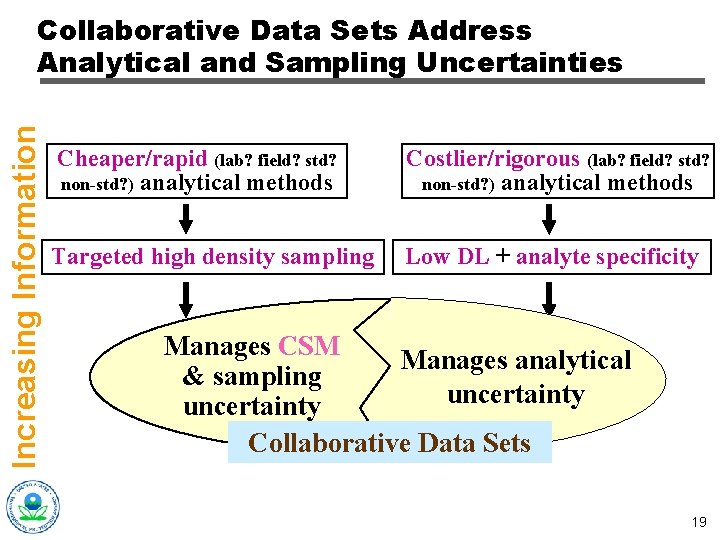
Increasing Information Collaborative Data Sets Address Analytical and Sampling Uncertainties Cheaper/rapid (lab? field? std? non-std? ) analytical methods Costlier/rigorous (lab? field? std? non-std? ) analytical methods Targeted high density sampling Low DL + analyte specificity Manages CSM Manages analytical & sampling uncertainty Collaborative Data Sets 19

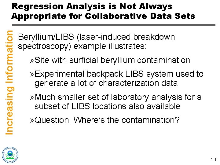
Increasing Information Regression Analysis is Not Always Appropriate for Collaborative Data Sets Beryllium/LIBS (laser-induced breakdown spectroscopy) example illustrates: » Site with surficial beryllium contamination » Experimental backpack LIBS system used to generate a lot of characterization data » Much smaller set of laboratory analysis for a subset of LIBS locations also available » Question: Where’s the contamination? 20

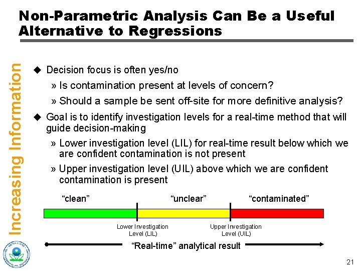
Increasing Information Non-Parametric Analysis Can Be a Useful Alternative to Regressions u Decision focus is often yes/no » Is contamination present at levels of concern? » Should a sample be sent off-site for more definitive analysis? u Goal is to identify investigation levels for a real-time method that will guide decision-making » Lower investigation level (LIL) for real-time result below which we are confident contamination is not present » Upper investigation level (UIL) above which we are confident contamination is present “clean” “unclear” Lower Investigation Level (LIL) “contaminated” Upper Investigation Level (UIL) “Real-time” analytical result 21

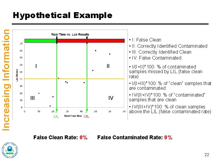
Increasing Information Hypothetical Example • I: False Clean • II: Correctly Identified Contaminated • III: Correctly Identified Clean • IV: False Contaminated I II IV IL LIL IL UIL False Clean Rate: 0% 25% • I/(I+II)*100: % of contaminated samples missed by LIL (false clean rate) • I/(I+III)*100: % of “clean” samples that are contaminated • IV/(II+IV)*100: % of “contaminated” samples that are clean • IV/(III+IV)*100: % of clean samples above the LIL (false contaminated rate) False Contaminated Rate: 0% 50% 22

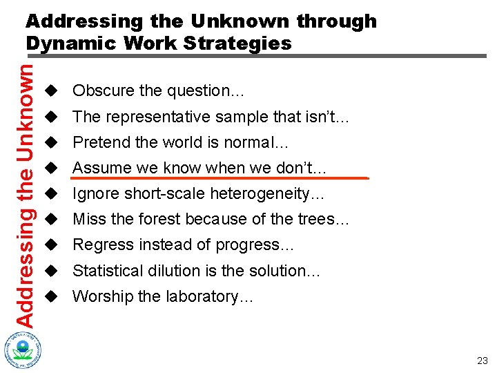
Addressing the Unknown through Dynamic Work Strategies u Obscure the question… u The representative sample that isn’t… u Pretend the world is normal… u Assume we know when we don’t… u Ignore short-scale heterogeneity… u Miss the forest because of the trees… u Regress instead of progress… u Statistical dilution is the solution… u Worship the laboratory… 23

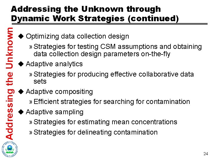
Addressing the Unknown through Dynamic Work Strategies (continued) u Optimizing data collection design » Strategies for testing CSM assumptions and obtaining data collection design parameters on-the-fly u Adaptive analytics » Strategies for producing effective collaborative data sets u Adaptive compositing » Efficient strategies for searching for contamination u Adaptive sampling » Strategies for estimating mean concentrations » Strategies for delineating contamination 24

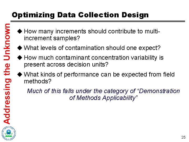
Addressing the Unknown Optimizing Data Collection Design u How many increments should contribute to multi- increment samples? u What levels of contamination should one expect? u How much contaminant concentration variability is present across decision units? u What kinds of performance can be expected from field methods? Much of this falls under the category of “Demonstration of Methods Applicability” 25

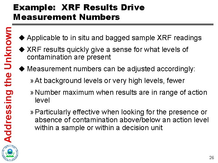
Addressing the Unknown Example: XRF Results Drive Measurement Numbers u Applicable to in situ and bagged sample XRF readings u XRF results quickly give a sense for what levels of contamination are present u Measurement numbers can be adjusted accordingly: » At background levels or very high levels, fewer » Number maximum when results are in range of action level » Particularly effective when looking for the presence or absence of contamination above/below an action level within a sample or within a decision unit 26

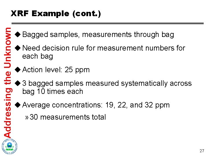
Addressing the Unknown XRF Example (cont. ) u Bagged samples, measurements through bag u Need decision rule for measurement numbers for each bag u Action level: 25 ppm u 3 bagged samples measured systematically across bag 10 times each u Average concentrations: 19, 22, and 32 ppm » 30 measurements total 27

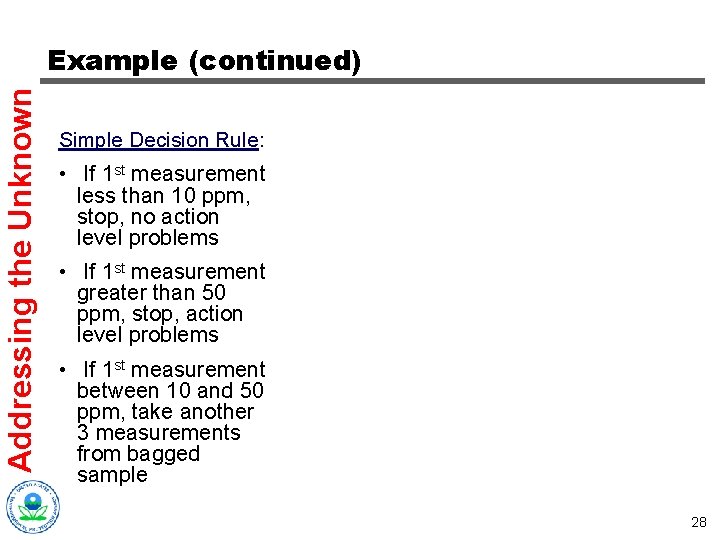
Addressing the Unknown Example (continued) Simple Decision Rule: • If 1 st measurement less than 10 ppm, stop, no action level problems • If 1 st measurement greater than 50 ppm, stop, action level problems • If 1 st measurement between 10 and 50 ppm, take another 3 measurements from bagged sample 28

Addressing the Unknown Adaptive Analytics u Goal is to identify elevated areas or delineate contamination u Assumptions: » Two methods, one cheap/less accurate, one expensive/“definitive” » Investigation levels (i. e. , LIL and UIL) can be derived for cheaper, real-time data u High density real-time data used to screen out areas that are obviously contaminated, or obviously clean u Fixed laboratory analyses target locations where real-time results were ambiguous u Design requires determining appropriate real-time investigation levels (e. g. , LIL and UIL) 29

Addressing the Unknown Adaptive Compositing Strategies u Goal: Identify elevated areas (or clear areas of contamination concerns) u Assumptions: » Contamination is believed to be spotty » Action level is significantly greater than background levels » Sample acquisition/handling costs are significantly less than analytical costs » Appropriate methods exist for sample acquisition and aggregation u Aggregate samples (single or multi-increment) into larger composites u Design requires determining the appropriate number of samples to composite, and developing decision criteria for composites that indicate when analyses of contributing multi-increment samples are necessary 30

Addressing the Unknown Recipe for Adaptive Compositing: u Determine appropriate number of samples to composite and resulting decision criteria. u Decision criteria = (action level - background)/(# of samples in composite) + background. u Sample and split samples. Use one set of splits to composite and save other set. u If: » composite result < decision criteria, done. » composite result > decision criteria, analyze splits contributing to composite. 31

Addressing the Unknown Example Decision Criteria u Background: 10 ppm; Action Level: 100 ppm u Determine decision criteria for 2 -sample, 3 -sample, 4 - sample, 5 -sample, and 6 -sample composite: » 2 -sample composite: 55 ppm » 3 -sample composite: 40 ppm » 4 -sample composite: 33 ppm » 5 -sample composite: 28 ppm » 6 -sample composite: 25 ppm 32

Addressing the Unknown When is Adaptive Compositing Cost. Effective? u The “spottier” contamination is, the better the performance u The greater the difference is between background and the action level, the better the performance u The greater the difference between the action level and average contamination concentration, the better the performance u Best case: no composite requires re-analysis u Worst case: every composite requires re-analysis 33

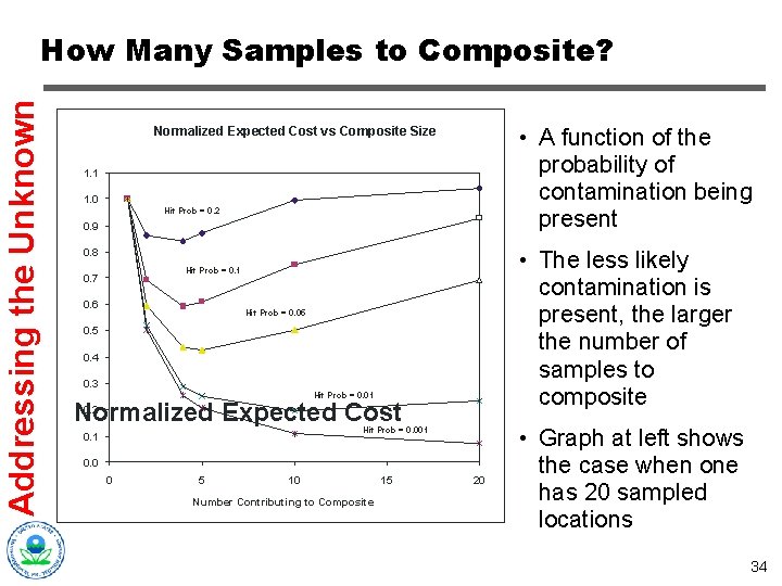
Addressing the Unknown How Many Samples to Composite? • A function of the probability of contamination being present Normalized Expected Cost vs Composite Size 1. 1 1. 0 Hit Prob = 0. 2 0. 9 0. 8 • The less likely contamination is present, the larger the number of samples to composite Hit Prob = 0. 1 0. 7 0. 6 Hit Prob = 0. 05 0. 4 0. 3 Hit Prob = 0. 01 0. 2 Normalized Expected Cost Hit Prob = 0. 001 0. 0 0 5 10 Number Contributing to Composite 15 20 • Graph at left shows the case when one has 20 sampled locations 34

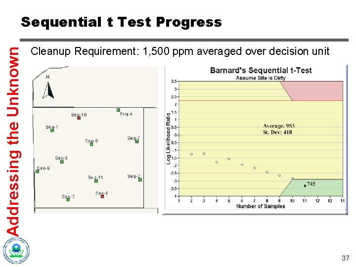
Addressing the Unknown Barnard’s Sequential t Test u This statistical test is the adaptive or sequential alternative to a one-sample Student t test, used to determine if the mean concentration in a decision unit is above or below a cleanup standard. u Sequential sampling-data evaluation-resampling… continue until the calculated average concentration is statistically either above the cleanup standard (site is “dirty”), or below the lower bound of the statistical gray region (site can be called “clean”) u Implementation requires some means for computing the required statistics. VSP has a Sequential t Test module that can do so. u For reference on “gray region: ” see EPA QA/G-4 2006, p. 53 35

Addressing the Unknown Barnard’s Sequential t Test (continued) u GOAL: Determine if mean concentration is above or below the conc. standard for a decision unit. u ASSUMPTIONS: » Underlying contamination is normally distributed. » You can specify some cut-off value (below the AL) that represents “definitely clean. ” In other words, if the average conc falls below the cut-off value, sampling can stop & the decision unit declared “clean” (this sets the lower bound of the gray region) » You can specify acceptable decision error (false clean & false dirty) rates. » A real-time quantitative method exists to provide unbiased data. » At least 10 samples will be collected if the degree of site heterogeneity (measured by variance or SD) is unknown. » Have some means for selecting the next sample locations in the sequence (e. g. , adaptive fill techniques) 36

Addressing the Unknown Sequential t Test Progress Cleanup Requirement: 1, 500 ppm averaged over decision unit 37

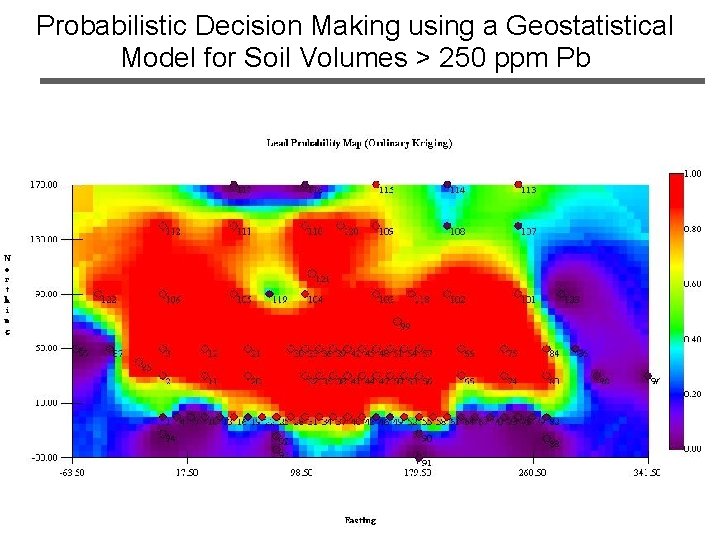
Probabilistic Decision Making using a Geostatistical Model for Soil Volumes > 250 ppm Pb Color coding for probabilities that 1 -ft deep ppm Pb (actual Pb conc not shown) volumes > 250 Decision plan: Will landfill any soil with Pr (Pb > 250 ppm) > 40%. Soil with Pr (Pb > 250 ppm) < 40% will be reused in new firing berm. 38

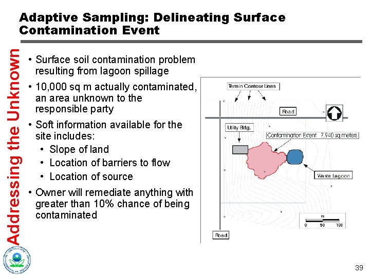
Addressing the Unknown Adaptive Sampling: Delineating Surface Contamination Event • Surface soil contamination problem resulting from lagoon spillage • 10, 000 sq m actually contaminated, an area unknown to the responsible party • Soft information available for the site includes: • Slope of land • Location of barriers to flow • Location of source • Owner will remediate anything with greater than 10% chance of being contaminated 39

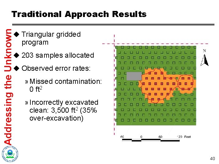
Addressing the Unknown Traditional Approach Results u Triangular gridded program u 203 samples allocated u Observed error rates: » Missed contamination: 0 ft 2 » Incorrectly excavated clean: 3, 500 ft 2 (35% over-excavation) 40

Addressing the Unknown Adaptive Cluster Sampling u GOAL: Determine average contaminant concentration over an area & delineate contamination footprints if any are found. u Assumptions: » The underlying distribution is normally distributed » Contamination likely has a well-defined footprint » Have quantitative, unbiased real-time analytics » Can designate what concentration constitutes a hot spot requiring delineation » Can lay a master grid over the area that encompasses all potential sampling points 41

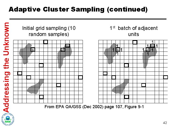
Addressing the Unknown Adaptive Cluster Sampling (continued) Initial grid sampling (10 random samples) 1 st batch of adjacent units From EPA QA/G 5 S (Dec 2002) page 107, Figure 9 -1 42

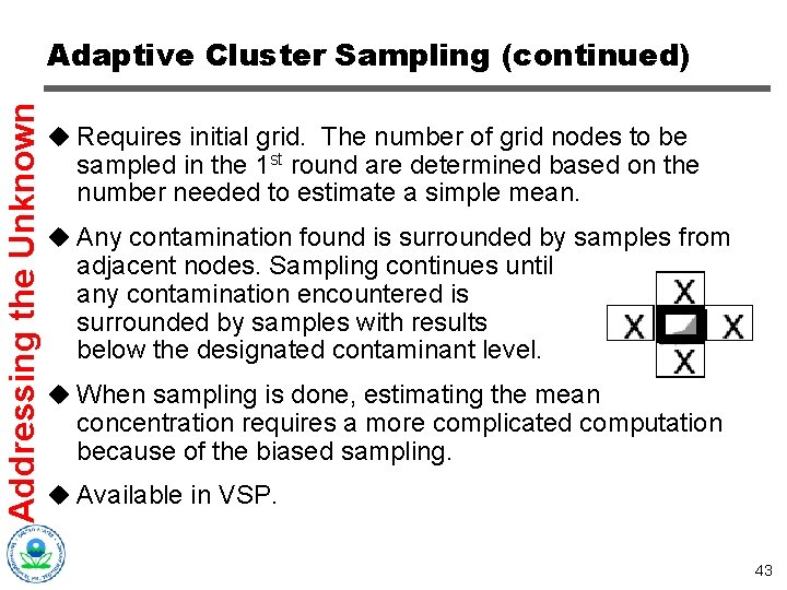
Addressing the Unknown Adaptive Cluster Sampling (continued) u Requires initial grid. The number of grid nodes to be sampled in the 1 st round are determined based on the number needed to estimate a simple mean. u Any contamination found is surrounded by samples from adjacent nodes. Sampling continues until any contamination encountered is surrounded by samples with results below the designated contaminant level. u When sampling is done, estimating the mean concentration requires a more complicated computation because of the biased sampling. u Available in VSP. 43

From EPA QA/G 5 S (Dec 2002) page 107 Figure 9 -1 Addressing the Unknown Adaptive Cluster Sampling (continued) 44

Addressing the Unknown Recipe for Adaptive Cluster Sampling u Lay master grid over site. u Start with an initial set of gridded samples, either determined by hot spot detection design or by design to estimate conc mean. u For every sample that is a hit, sample neighboring grid nodes. u Continue until no more hits are encountered. u Complicated calculations: use VSP to calculate the mean estimate and associated confidence interval. 45

Addressing the Unknown Recipe: u Lay master grid over site. u Start with an initial set of gridded samples, either determined by hot spot analysis or sample mean analysis. u For every sample that is a hit, sample neighboring grid nodes. u Continue until no more hits are encountered. u Use VSP to determine mean estimate and associated confidence interval. 46

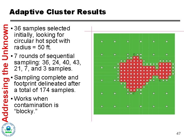
Addressing the Unknown Adaptive Cluster Results • 36 samples selected initially, looking for circular hot spot with radius = 50 ft. • 7 rounds of sequential sampling: 36, 24, 40, 43, 21, 7, and 3 samples. • Sampling complete and footprint delineated after a total of 174 samples. • Works when contamination is “blocky. ” 47

Addressing the Unknown Adaptive Geo. Bayesian Approaches u Goal: Hot spots and boundary delineation u Assumptions: » Appropriate real-time technique is available » Yes/no sample results » Spatial autocorrelation is significant » Desire to leverage collaborative information u Method uses geostatistics & Bayesian analysis of collaborative data to guide sampling program & estimate probability of contamination at any location. u Must have appropriate investigation levels for real-time technique & estimate of spatial autocorrelation range. Mean estimates can be obtained using block kriging. u Available in BAASS software (contact Bob Johnson, ANL) 48

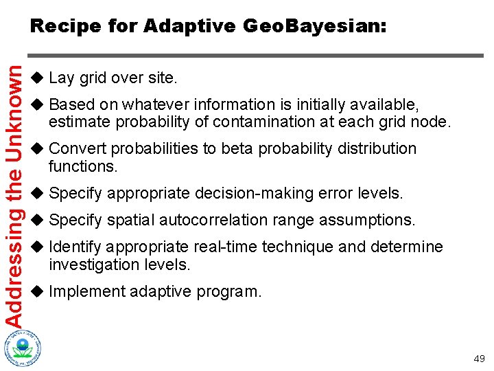
Addressing the Unknown Recipe for Adaptive Geo. Bayesian: u Lay grid over site. u Based on whatever information is initially available, estimate probability of contamination at each grid node. u Convert probabilities to beta probability distribution functions. u Specify appropriate decision-making error levels. u Specify spatial autocorrelation range assumptions. u Identify appropriate real-time technique and determine investigation levels. u Implement adaptive program. 49

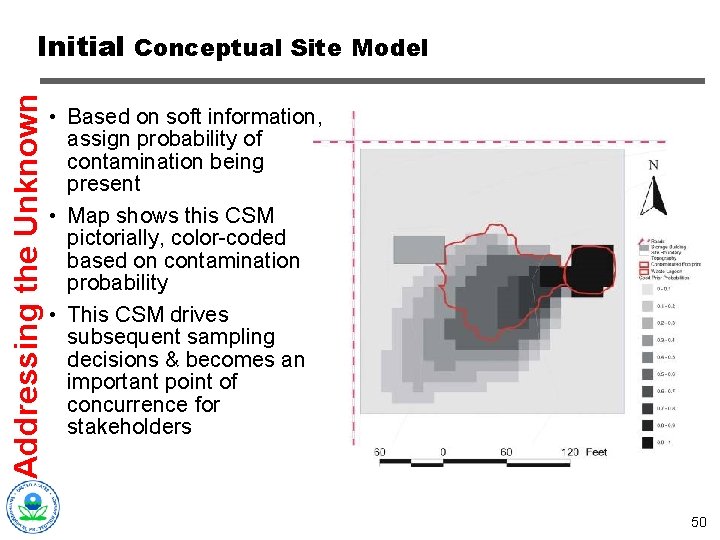
Addressing the Unknown Initial Conceptual Site Model • Based on soft information, assign probability of contamination being present • Map shows this CSM pictorially, color-coded based on contamination probability • This CSM drives subsequent sampling decisions & becomes an important point of concurrence for stakeholders 50

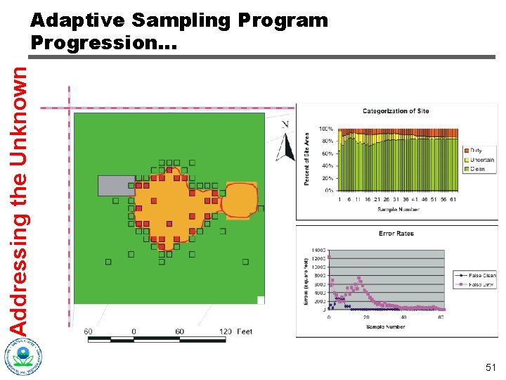
Addressing the Unknown Adaptive Sampling Program Progression… 51

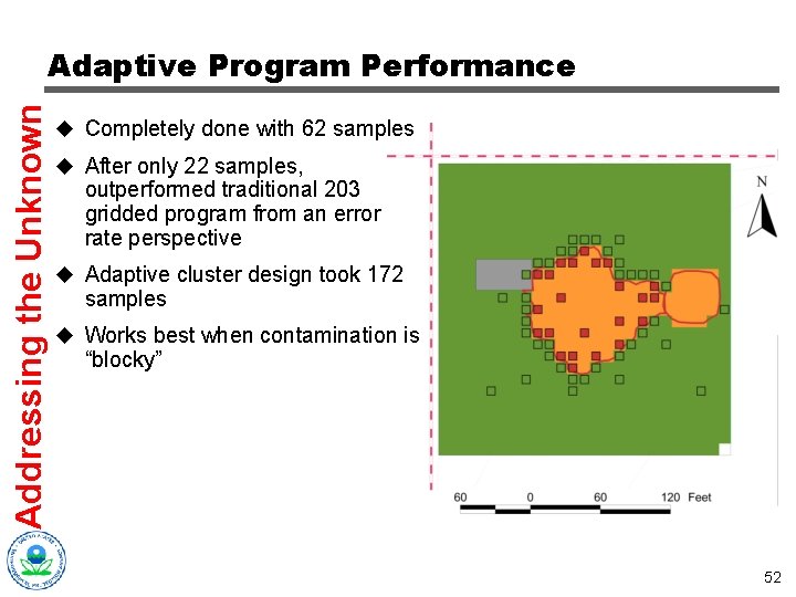
Addressing the Unknown Adaptive Program Performance u Completely done with 62 samples u After only 22 samples, outperformed traditional 203 gridded program from an error rate perspective u Adaptive cluster design took 172 samples u Works best when contamination is “blocky” 52

The Biggest Bang Comes from Combining… u CSM knowledge, with… u Multi-increment sampling, with… u Collaborative data sets, with… u Adaptive analytics, with… u Adaptive QC & data uncertainty reduction, with… u Adaptive compositing, with… u Adaptive sample location selection. 53