S 519 Evaluation of Information Systems Social Statistics

S 519: Evaluation of Information Systems Social Statistics Inferential Statistics Chapter 8: Significantly significant

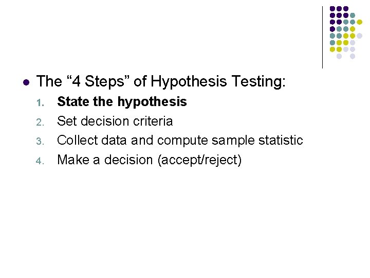
l The “ 4 Steps” of Hypothesis Testing: 1. 2. 3. 4. State the hypothesis Set decision criteria Collect data and compute sample statistic Make a decision (accept/reject)

This week l l Types of variables Central Limit Theorem Steps of hypothesis testing Type I and Type II errors

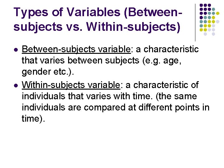
Types of Variables (Betweensubjects vs. Within-subjects) l l Between-subjects variable: a characteristic that varies between subjects (e. g. age, gender etc. ). Within-subjects variable: a characteristic of individuals that varies with time. (the same individuals are compared at different points in time).

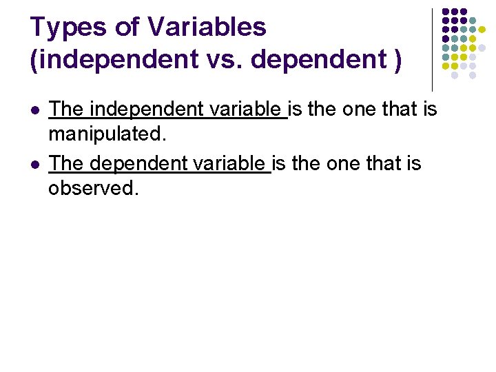
Types of Variables (independent vs. dependent ) l l The independent variable is the one that is manipulated. The dependent variable is the one that is observed.

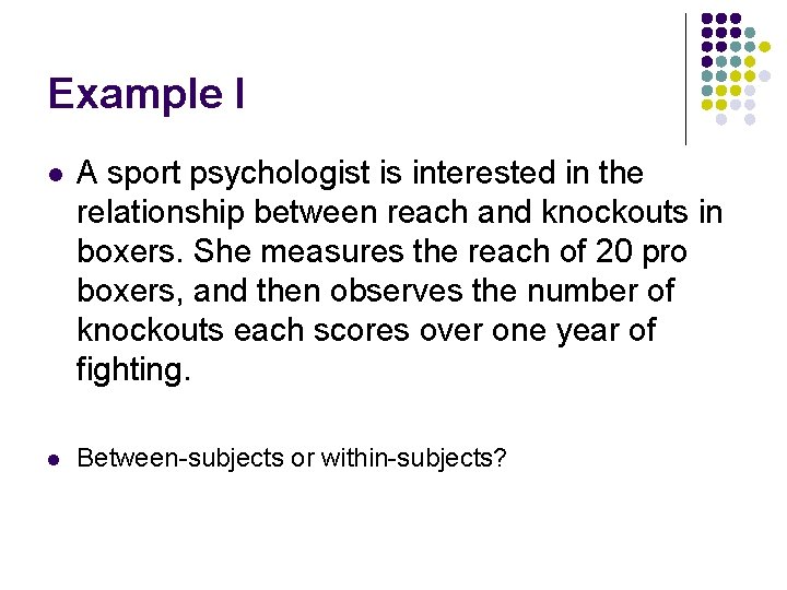
Example I l A sport psychologist is interested in the relationship between reach and knockouts in boxers. She measures the reach of 20 pro boxers, and then observes the number of knockouts each scores over one year of fighting. l Between-subjects or within-subjects?

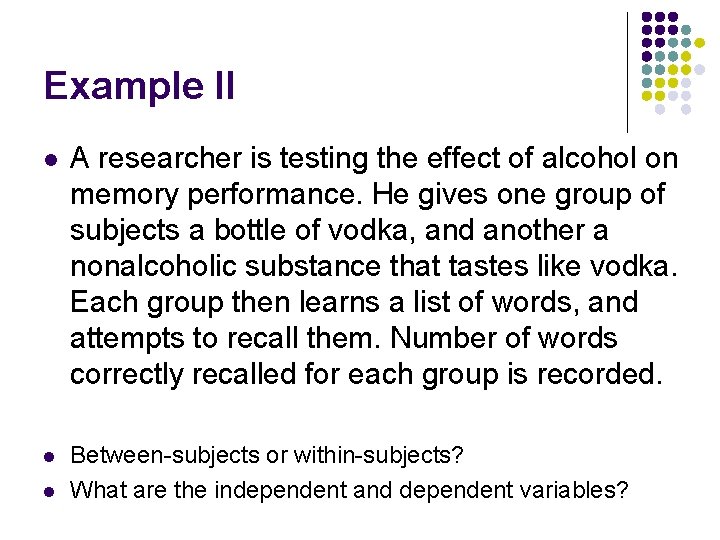
Example II l A researcher is testing the effect of alcohol on memory performance. He gives one group of subjects a bottle of vodka, and another a nonalcoholic substance that tastes like vodka. Each group then learns a list of words, and attempts to recall them. Number of words correctly recalled for each group is recorded. l Between-subjects or within-subjects? What are the independent and dependent variables? l

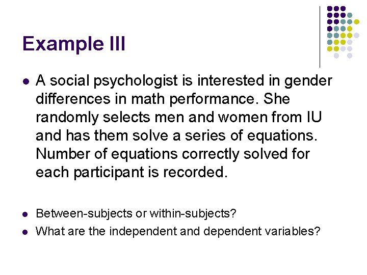
Example III l A social psychologist is interested in gender differences in math performance. She randomly selects men and women from IU and has them solve a series of equations. Number of equations correctly solved for each participant is recorded. l Between-subjects or within-subjects? What are the independent and dependent variables? l

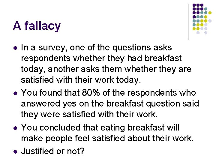
A fallacy l l In a survey, one of the questions asks respondents whether they had breakfast today, another asks them whether they are satisfied with their work today. You found that 80% of the respondents who answered yes on the breakfast question said they were satisfied with their work. You concluded that eating breakfast will make people feel satisfied about their work. Justified or not?

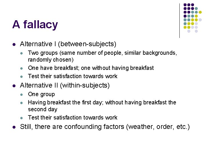
A fallacy l Alternative I (between-subjects) l l Alternative II (within-subjects) l l Two groups (same number of people, similar backgrounds, randomly chosen) One have breakfast; one without having breakfast Test their satisfaction towards work One group Having breakfast the first day; without having breakfast the second day Test their satisfaction towards work Still, there are confounding factors (weather, order, etc. )

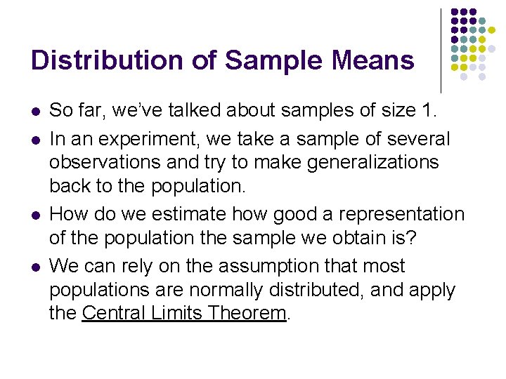
Distribution of Sample Means l l So far, we’ve talked about samples of size 1. In an experiment, we take a sample of several observations and try to make generalizations back to the population. How do we estimate how good a representation of the population the sample we obtain is? We can rely on the assumption that most populations are normally distributed, and apply the Central Limits Theorem.

Sampling Distributions l The distribution of sample means contains all sample means of a size n that can be obtained from a population.

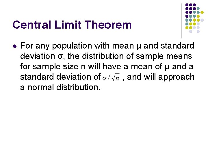
Central Limit Theorem l For any population with mean μ and standard deviation σ, the distribution of sample means for sample size n will have a mean of μ and a standard deviation of , and will approach a normal distribution.

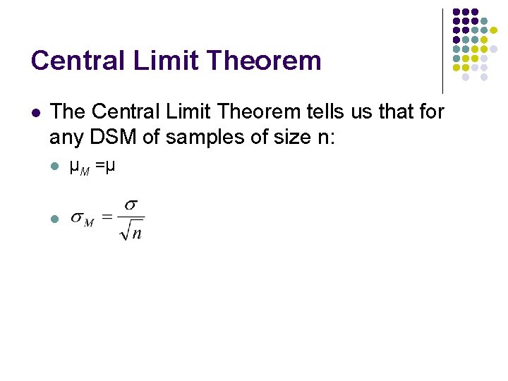
Central Limit Theorem l The Central Limit Theorem tells us that for any DSM of samples of size n: l l μM =μ

Central Limit Theorem l l The mean of the distribution of sample means is called the expected value of M. The standard deviation of the distribution of sample means is called the standard error of M. standard error = σM Standard deviation: standard distance between a score X and the population mean μ. Standard error: standard distance between a sample mean M and the population mean μ.

Probability and the Sample Means Distribution l l l SAT-scores (μ=500, σ=100). What is the probability (M>540)? If l l Choose one randomly from the population; Take sample n=25.

Step 1: State Hypothesis l Hypothesis is stated in terms of a population parameter (e. g. μ): assume null unless sufficient evidence to reject it l l Null Hypothesis: no change in population parameter, treatment has no effect. H 0 Alternate (Scientific) Hypothesis: opposite of H 0, treatment has an effect. H 1 (directional or non directional)

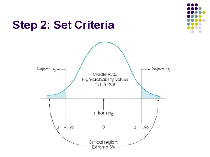
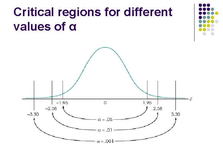
Step 2: Set Criteria l l l By selecting a probability value (level of significance or alpha level), e. g. α = 0. 05, 0. 01, 0. 001 Critical region is region of extreme sample values (unlikely to be obtained if H 0 is true). If sample data fall within the critical region, H 0 is rejected. Determine exact values for boundaries of critical region by using α and unit normal table.

Step 2: Set Criteria

Step 3: Collect Data/Statistics l l Select random sample and perform “experiment”. Compute sample statistic, e. g. sample mean. Locate sample statistic within hypothesized distribution (use z-score). Is sample statistic located within the critical region?

Step 4: Decision l l Possibility: sample statistic is within critical region. Reject H 0. Possibility: sample statistic is not within critical region. Do not reject H 0.

Hypothesis Testing: An Example l l l It is known that corn in Bloomington grows to an average height of μ=72 σ=6 six months after being planted. We are studying the effect of “Plant Food 6000” on corn growth. We randomly select a sample of 40 seeds from the above population and plant them, using PF-6000 each week for six months. At the end of the six month period, our sample has a height of M=78 inches. Go through the steps of hypothesis testing and draw a conclusion about PF-6000 1. State hypotheses; 2. Chance model/critical region; 3. Collect data; 4. Decision and conclusion

Step 1: State Hypotheses l In words l l l Null: PF 6000 will not have an effect on corn growth Alt: PF 6000 will have an effect on corn growth In “code” symbols: l l H 0 : μ = 72 H 1 : μ ≠ 72

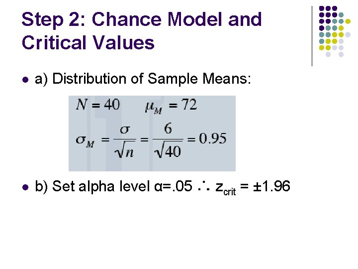
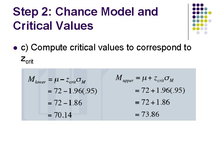
Step 2: Chance Model and Critical Values l a) Distribution of Sample Means: l b) Set alpha level α=. 05 ∴ zcrit = ± 1. 96

Step 2: Chance Model and Critical Values l c) Compute critical values to correspond to zcrit

Step 3: Do Experiment l For the question, this part has already been done for us, we just need to compare this obtained sample mean to our chance model to determine if any discrepancy between our sample and the original population is due to: l l 1. Sampling Error 2. A true effect of our manipulation

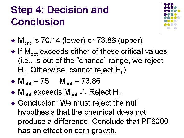
Step 4: Decision and Conclusion l l l Mcrit is 70. 14 (lower) or 73. 86 (upper) If Mobt exceeds either of these critical values (i. e. , is out of the “chance” range, we reject H 0. Otherwise, cannot reject H 0) Mobt = 78 Mcrit = 73. 86 Mobt exceeds Mcrit ∴ Reject H 0 Conclusion: We must reject the null hypothesis that the chemical does not produce a difference. Conclude that PF 6000 has an effect on corn growth.

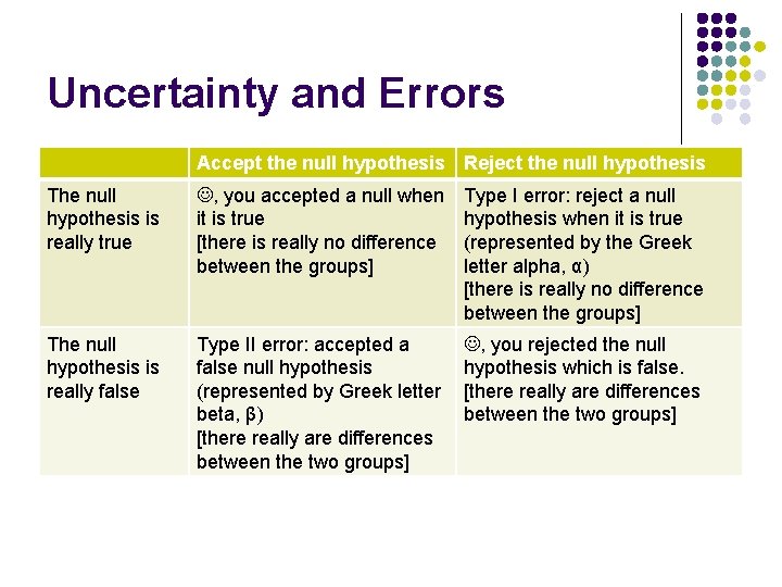
Uncertainty and Errors Accept the null hypothesis Reject the null hypothesis The null hypothesis is really true , you accepted a null when it is true [there is really no difference between the groups] Type I error: reject a null hypothesis when it is true (represented by the Greek letter alpha, α) [there is really no difference between the groups] The null hypothesis is really false Type II error: accepted a false null hypothesis (represented by Greek letter beta, β) [there really are differences between the two groups] , you rejected the null hypothesis which is false. [there really are differences between the two groups]

Critical regions for different values of α

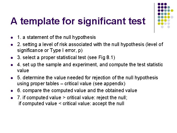
A template for significant test l l l l 1. a statement of the null hypothesis 2. setting a level of risk associated with the null hypothesis (level of significance or Type I error, p) 3. select a proper statistical test (see Fig 8. 1) 4. set up the sample and experiment, and compute the test statistic value 5. determine the value needed for rejection of the null hypothesis using proper tables – critical value (see appendix) 6. compare the computed value and the obtained value 7. if computed value > critical value: reject the null; if computed value < critical value: accept the null